

Advanced Study Material for Class 11 Physics: Chapter 01 Units and Measurement
Access comprehensive study materials and useful resources for Chapter 01 Units and Measurement using the CBSE Class 11 Physics Units Dimensions Vectors Exam Notes. Designed to align with the 2026-27 CBSE academic guidelines, these advanced resources help Class 11 Physics students reinforce core concepts beyond standard textbooks.
Practice Class 11 Physics Resources: Chapter 01 Units and Measurement
Access the complete useful resource PDF for Class 11 Physics below. Regular practice with these targeted academic notes builds familiarity with complex topics and helps secure higher marks in final school evaluations.
CBSE Class 12 Physics: Units, Dimensions & Vectors Exam Notes
UNITS, DIMENSIONS & VECTORS
UNITS AND DIMENSIONS
In order to measure a physical quantity, it has to be expressed in terms of a certain reference standard of measurement of that physical quantity, which is called a unit. The magnitude of a physical quantity is expressed in terms of the number of times the physical quantity contains that unit.
The basic physical quantities, which do not depend upon other quantities, are known as the fundamental quantities. Mass, length and time are considered as fundamental quantities. The units which can be derived from the fundamental units are known as derived units. In mechanics, all quantities can be expressed in terms of mass, length and time. The main systems of units are given as follows:
- C.G.S. or Centimetre, Gram, Second system.
- F.P.S. or Foot, Pound, Second system.
- M.K.S. or Metre, Kilogram, Second system.
- S.I. system: There are seven basic or fundamental quantities in the International System of Units, called the S.I. system, which can express all physical quantities including heat, optics, electricity and magnetism. These seven basic quantities with their units and symbols are given as follows:
| S.No. | Physical quantity | S.I. unit | Symbol |
|---|---|---|---|
| 1 | Mass | Kilogram | kg |
| 2 | Length | Metre | m |
| 3 | Time | Second | s |
| 4 | Temperature | Kelvin | K |
| 5 | Luminous intensity | Candela | cd |
| 6 | Electric current | Ampere | A |
| 7 | Amount of substance | Mole | mol |
Also, two supplementary units are used: the radian (rad) for plane angle and the steradian (sr) for solid angle.
The International System of Units (S.I.) is now extensively used for scientific measurements.
The following practical units are conveniently used and are expressed in terms of the S.I. system of units also.
- Micron is a small unit for measurement of length. 1 micron = 1 \(\mu\)m = \(10^{-6}\) m.
- Angstrom is a unit of length in which the size of an atom is measured and is used in atomic physics. 1 Angstrom = 1 Å = \(10^{-10}\) m.
- Light year is a unit of distance travelled by light in free space and is used in astrophysics. \[ 1\ \text{light year}=3\times10^8\ \text{m/s}\times365\times24\times60\times60\ \text{s}=9.5\times10^{15}\ \text{m} \]
- Fermi is a unit of distance in which the size of a nucleus is measured. 1 Fermi = \(10^{-15}\) m.
- Atomic mass unit is a unit of mass equal to 1/12th of the mass of a carbon-12 nucleus and is used in measuring the masses of nuclei. 1 atomic mass unit \(\approx1.67\times10^{-27}\) kg.
DIMENSIONS
The dimensions of a physical quantity are the powers to which the fundamental units of mass, length and time should be raised to represent that physical quantity. The expression which represents the dimensions of a physical quantity is called the dimensional formula, which is given as \([M^aL^bT^c]\), where \(a\), \(b\) and \(c\) are the respective dimensions of mass, length and time.
For example, the dimensional formula for volume = \([L^3]\), velocity = \([LT^{-1}]\), power = \([ML^2T^{-2}]\), etc.
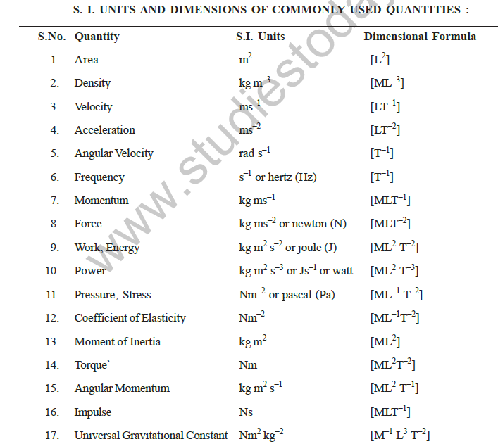
S.I. units and dimensions of commonly used quantities:
| S.No. | Quantity | S.I. units | Dimensional formula |
|---|---|---|---|
| 1 | Area | m2 | \([L^2]\) |
| 2 | Density | kg m−3 | \([ML^{-3}]\) |
| 3 | Velocity | m s−1 | \([LT^{-1}]\) |
| 4 | Acceleration | m s−2 | \([LT^{-2}]\) |
| 5 | Angular velocity | rad s−1 | \([T^{-1}]\) |
| 6 | Frequency | s−1 or hertz (Hz) | \([T^{-1}]\) |
| 7 | Momentum | kg m s−1 | \([MLT^{-1}]\) |
| 8 | Force | kg m s−2 or newton (N) | \([MLT^{-2}]\) |
| 9 | Work, energy | kg m2 s−2 or joule (J) | \([ML^2T^{-2}]\) |
| 10 | Power | kg m2 s−3 or J s−1 or watt | \([ML^2T^{-3}]\) |
| 11 | Pressure, stress | N m−2 or pascal (Pa) | \([ML^{-1}T^{-2}]\) |
| 12 | Coefficient of elasticity | N m−2 | \([ML^{-1}T^{-2}]\) |
| 13 | Moment of inertia | kg m2 | \([ML^2]\) |
| 14 | Torque | N m | \([ML^2T^{-2}]\) |
| 15 | Angular momentum | kg m2 s−1 | \([ML^2T^{-1}]\) |
| 16 | Impulse | N s | \([MLT^{-1}]\) |
| 17 | Universal gravitational constant | N m2 kg−2 | \([M^{-1}L^3T^{-2}]\) |
| 18 | Latent heat | J kg−1 | \([L^2T^{-2}]\) |
| 19 | Specific heat | J kg−1 K−1 | \([L^2T^{-2}K^{-1}]\) |
| 20 | Thermal conductivity | J m−1 s−1 K−1 | \([MLT^{-3}K^{-1}]\) |
| 21 | Electric charge | coulomb (C) | \([AT]\) |
| 22 | Electric potential | J C−1 or volt (V) | \([ML^2T^{-3}A^{-1}]\) |
| 23 | Electric resistance | V A−1 or ohm (Ω) | \([ML^2T^{-3}A^{-2}]\) |
| 24 | Electric resistivity | Ω m | \([ML^3T^{-3}A^{-2}]\) |
| 25 | Capacitance | C V−1 or farad (F) | \([M^{-1}L^{-2}T^4A^2]\) |
| 26 | Inductance | V s A−1 or henry (H) | \([ML^2T^{-2}A^{-2}]\) |
| 27 | Electric field | N C−1 or V m−1 | \([MLT^{-3}A^{-1}]\) |
| 28 | Magnetic induction | N A−1 m−1 or tesla (T) | \([MT^{-2}A^{-1}]\) |
| 29 | Magnetic flux | T m2 or weber (Wb) | \([ML^2T^{-2}A^{-1}]\) |
| 30 | Permittivity | C2 N−1 m−2 | \([M^{-1}L^{-3}T^4A^2]\) |
| 31 | Permeability | T m A−1 or Wb A−1 m−1 | \([MLT^{-2}A^{-2}]\) |
| 32 | Planck’s constant | J s | \([ML^2T^{-1}]\) |
| 33 | Boltzmann constant | J K−1 | \([ML^2T^{-2}K^{-1}]\) |
USES OF DIMENSIONAL EQUATION
- Conversion of one system of units into another. If \(n_1\) is the numerical value of a physical quantity with dimensions \(a\), \(b\) and \(c\) for units of mass, length and time \(M_1\), \(L_1\) and \(T_1\), the numerical value \(n_2\) of the same quantity for different units of mass, length and time \(M_2\), \(L_2\) and \(T_2\) respectively can be calculated as \[ n_2=n_1\left[\frac{M_1}{M_2}\right]^a\left[\frac{L_1}{L_2}\right]^b\left[\frac{T_1}{T_2}\right]^c \]
- To test the correctness of a physical equation or formula. The principle of homogeneity requires that the dimensions of all the terms on both sides of a physical equation or formula should be equal if the physical equation or any derived formula is correct.
- To derive a relation between different physical quantities in any physical phenomenon. If a physical quantity depends upon a number of parameters whose dimensions are not known, the principle of homogeneity of dimensions can be used. As the dimensions of a correct dimensional equation are equal on both sides, it can be used to find the unknown dimensions of the parameters on which the physical quantity depends. It can be used to derive the relations between any physical quantity and its dependent parameters.
LIMITATIONS OF DIMENSIONAL EQUATION
- From a dimensional equation, the nature of physical quantities cannot be decided, i.e., whether a given quantity is scalar or vector.
- The value of the constant of proportionality cannot be determined.
- Relations among physical quantities having exponential, logarithmic and trigonometric functions cannot be established.
- A relation which depends on more than three physical quantities in mechanics, and on more than four physical quantities in current electricity, cannot be established; however, its validity can be checked.
- Relations which are in more than one part cannot be determined.
VECTORS
Scalars: Quantities having only magnitude, no direction, and obeying the algebraic law of addition are said to be scalars. Mathematically, algebraic addition is represented as \(a+b=c\).
Examples of scalar quantities are mass, length, time, distance, speed, work, energy, power, gravitational potential, electric potential, electric flux, magnetic flux, current, etc.
Vectors: Quantities having magnitude and direction and obeying the triangle law of vector addition are said to be vectors. Mathematically, the triangle law is represented as \(\vec a+\vec b=\vec c\).
Examples of vector quantities are displacement, velocity, momentum, force, torque, acceleration, electric field strength, magnetic field strength, electric dipole moment, magnetic dipole moment, etc.
Representation of a vector:
- O → initial point or tail of a vector.
- A → final point or head of a vector.
- \(\vec a\) → a vector whose magnitude is proportional to the length of the straight line OA and whose direction is from O to A.
- \(-\vec a\) → a vector whose magnitude is equal to that of vector \(\vec a\) but whose direction is opposite.
Addition of vectors
Consider vectors \(\vec A\) and \(\vec B\) with magnitudes \(A\) and \(B\) respectively. If a line drawn from point O to P represents \(\vec A\), the second vector \(\vec B\) is drawn from the head of \(\vec A\), i.e., from point P along PQ, which is parallel to \(\vec B\). The resultant \(\vec R\) is represented by OQ by applying the triangular law of addition of vectors. The law states that if two vectors are represented in magnitude and direction by the two sides of a triangle, the third side of the triangle, taken from the origin of the first vector, represents their resultant in magnitude and direction.
\[\vec R=\vec A+\vec B\]
The resultant \(\vec R\) of vectors \(\vec A\) and \(\vec B\) can also be found from the law of parallelogram of vectors, which states that if two vectors \(\vec A\) and \(\vec B\) are represented by two adjacent sides of a parallelogram pointing outwards, the diagonal drawn through the intersection of the two vectors represents the vector sum of the two vectors. If OP and OQ represent vectors \(\vec A\) and \(\vec B\) respectively at angle \(\theta\), their resultant \(\vec R\) along OM is given by
\[(OM)^2=(ON)^2+(MN)^2=(OP+PN)^2+(MN)^2\]
\[R^2=(A+B\cos\theta)^2+(B\sin\theta)^2=A^2+B^2+2AB\cos\theta\]
\[R=\left[A^2+B^2+2AB\cos\theta\right]^{1/2}\]
If \(\alpha\) is the angle subtended by the resultant \(\vec R\) with OP,
\[\tan\alpha=\frac{MN}{OP+PN}=\frac{B\sin\theta}{A+B\cos\theta}\ \Rightarrow\ \alpha=\tan^{-1}\left[\frac{B\sin\theta}{A+B\cos\theta}\right]\]
- If \(\vec A\) and \(\vec B\) are in the same direction, \(\theta=0^\circ\) and \(|\vec R|=A+B\).
- If \(\vec A\) and \(\vec B\) are in opposite directions, \(\theta=180^\circ\) and \(|\vec R|=A-B\).
- If \(\vec A\) and \(\vec B\) are perpendicular to each other, \(|\vec R|=\sqrt{A^2+B^2}\) and \(\alpha=\tan^{-1}\left(\dfrac BA\right)\).
The addition of vectors obeys the following laws:
- Commutative law: \(\vec A+\vec B=\vec B+\vec A\)
- Associative law: \((\vec A+\vec B)+\vec C=\vec A+(\vec B+\vec C)\)
- Distributive law: \((b+c)\vec A=b\vec A+c\vec A\), where \(b\) and \(c\) are scalar quantities.
SUBTRACTION OF VECTORS
The subtraction of a vector \(\vec B\) from the vector \(\vec A\) is equivalent to the addition of vector \(\vec A\) with \(-\vec B\), giving the resultant \(\vec R\) as
\[\vec R=\vec A-\vec B=\vec A+(-\vec B)\]
where \(-\vec B\) implies a vector of the magnitude of \(\vec B\) but of opposite direction.
RESOLUTION OF VECTORS
A vector \(\vec A\) with its tail at the origin of a two-dimensional coordinate system \((x,y)\) can be resolved into two components \(\vec A_x\) and \(\vec A_y\) by drawing perpendiculars from the head of vector \(\vec A\) on the \(x\) and \(y\) axes respectively. \(\vec A\) is resolved into two rectangular components \(\vec A_x\) and \(\vec A_y\).
\[\therefore\ \vec A=\vec A_x+\vec A_y\]
Let \(\hat i\) be a unit vector, i.e., of magnitude unity, directed along the \(x\)-axis and \(\hat j\) a unit vector of magnitude unity along the \(y\)-direction. If \(A_x\) and \(A_y\) are the magnitudes of vectors \(\vec A_x\) and \(\vec A_y\), then
\[\vec A_x=A_x\hat i\quad\text{and}\quad\vec A_y=A_y\hat j\]
Thus a vector \(\vec A\) can be written in the form of notation of unit vectors along the \(x\) and \(y\) axes as
\[\vec A=A_x\hat i+A_y\hat j\]
If \(\theta\) is the angle subtended by vector \(\vec A\) with the \(x\)-axis, \(A_x=A\cos\theta\) and \(A_y=A\sin\theta\) represent the rectangular components of \(\vec A\) along two perpendicular directions,
\[|\vec A|=\sqrt{A_x^2+A_y^2}=\sqrt{A^2\cos^2\theta+A^2\sin^2\theta}\]
\[\tan\theta=\frac{A_y}{A_x}\quad\text{or}\quad\theta=\tan^{-1}\left(\frac{A_y}{A_x}\right)\]
MULTIPLICATION OF VECTORS
1. Multiplication of a vector by a scalar: If a vector \(\vec A\) is multiplied by a scalar quantity \(c\), the result is a vector whose magnitude is \(c\) times the magnitude of \(\vec A\) and whose direction is the same as that of \(\vec A\).
2. Scalar or dot product: If the product of two vectors \(\vec A\) and \(\vec B\) is a scalar quantity, it is called the scalar or dot product, i.e., \(\vec A\cdot\vec B\). The scalar or dot product of two vectors is equal to the product of the magnitudes of the two vectors and the cosine of the angle between these vectors.
\[\vec A\cdot\vec B=A(B\cos\theta)=B(A\cos\theta)\]
The dot product of two vectors is the product of the magnitude of one vector and the magnitude of the component of the second vector along the direction of the first vector.
The work \(W\) done by a force \(\vec F\) to produce a displacement \(\vec S\) at an angle \(\theta\) to the direction of the force is given by
\[W=\vec F\cdot\vec S=FS\cos\theta\]
The dot product of perpendicular vectors is zero. The dot product of a vector with itself is equal to the square of its magnitude.
The scalar product of vectors obeys the following laws:
- Commutative law: \(\vec A\cdot\vec B=\vec B\cdot\vec A\)
- Distributive law: \(\vec A\cdot(\vec B+\vec C)=\vec A\cdot\vec B+\vec A\cdot\vec C\) and \(\vec A\cdot(\vec B-\vec C)=\vec A\cdot\vec B-\vec A\cdot\vec C\)
3. Vector or cross product: The vector or cross product of two vectors \(\vec A\) and \(\vec B\) is itself a vector and is denoted by \(\vec A\times\vec B\). The vector or cross product \(\vec R\) of two vectors has a magnitude equal to the product of the magnitudes of the two vectors and the sine of the smaller angle \(\theta\) between the two vectors.
\[\vec R=\vec A\times\vec B=AB\sin\theta\,\hat n\]
where \(\hat n\) is a unit vector perpendicular to the plane of \(\vec A\) and \(\vec B\). Here \(\theta\) is the smaller angle between \(\vec A\) and \(\vec B\) which is used, and not \((360^\circ-\theta)\), which is the larger angle between these vectors. The direction of the resultant vector product \(\vec A\times\vec B\) is given by the following rule:
RIGHT-HANDED THUMB RULE
If we bend the fingers of the right hand and curl them in such a way that they point in the direction of rotation from vector \(\vec A\) to vector \(\vec B\) through the smaller angle between them, the thumb of the right hand points in the direction of the resultant vector product \(\vec A\times\vec B\). The figure shows the fingers of the right hand curled from \(\vec A\) to \(\vec B\) in the anticlockwise direction.
The vector product or cross product of vectors obeys the following laws:
- Distributive law: \(\vec A\times(\vec B+\vec C)=\vec A\times\vec B+\vec A\times\vec C\) and \(\vec A\times(\vec B-\vec C)=\vec A\times\vec B-\vec A\times\vec C\)
- Null vectors: The vector product of two parallel vectors is a null vector. \[ \vec A\times\vec B=AB\sin0^\circ=0 \] Also the vector product of a vector by itself is a null vector: \[ \vec A\times\vec A=A\cdot A\sin0^\circ=0 \]
- The vector product of two vectors gives the area of the parallelogram formed by these two vectors.
- The vector product is non-commutative: \(\vec A\times\vec B\neq\vec B\times\vec A\), \(\vec A\times\vec B=-\vec B\times\vec A\).
For example, in rotatory motion, the torque \(\vec\tau\) acting on a body due to a force \(\vec F\) applied at a perpendicular distance \(\vec r\) from the axis of rotation is given by the cross product of these vectors, \(\vec\tau=\vec r\times\vec F\).
Angular momentum \(\vec L\) is related to linear momentum \(\vec p\) and radius \(\vec r\) as \(\vec L=\vec r\times\vec p\). The linear velocity \(\vec v\) in circular motion is related to the angular velocity \(\vec\omega\) and the radius \(\vec r\) of the circular path as \(\vec v=\vec r\times\vec\omega\).
THREE DIMENSIONAL VECTOR
If \(\vec A\) is a vector in space which has components \(A_x\), \(A_y\) and \(A_z\) along the three dimensions of the Cartesian system of coordinates \((x,y,z)\), \(\vec A\) can be written in the form of unit vector notation as
\[\vec A=A_x\hat i+A_y\hat j+A_z\hat k\]
where \(\hat i,\hat j,\hat k\) represent unit vectors in the positive directions of the \(x\), \(y\) and \(z\) axes respectively. Thus two vectors \(\vec A\) and \(\vec B\) can be written in the notation of unit vectors \(\hat i,\hat j,\hat k\) as follows:
\[\vec A=A_x\hat i+A_y\hat j+A_z\hat k,\qquad\vec B=B_x\hat i+B_y\hat j+B_z\hat k\]
\[\therefore\ \vec A+\vec B=(A_x+B_x)\hat i+(A_y+B_y)\hat j+(A_z+B_z)\hat k\]
Scalar product of vectors \(\vec A\) and \(\vec B\):
\[\vec A\cdot\vec B=(A_x\hat i+A_y\hat j+A_z\hat k)\cdot(B_x\hat i+B_y\hat j+B_z\hat k)=A_xB_x+A_yB_y+A_zB_z\]
since \(\hat i\cdot\hat j=\hat j\cdot\hat k=\hat k\cdot\hat i=0\) and \(\hat i\cdot\hat i=\hat j\cdot\hat j=\hat k\cdot\hat k=1\).
Vector product of vectors \(\vec A\) and \(\vec B\):
\[\vec A\times\vec B=(A_x\hat i+A_y\hat j+A_z\hat k)\times(B_x\hat i+B_y\hat j+B_z\hat k)\]
As \(\hat i\times\hat i=\hat j\times\hat j=\hat k\times\hat k=0\), and
\[\hat i\times\hat j=-\hat j\times\hat i=\hat k,\quad\hat j\times\hat k=-\hat k\times\hat j=\hat i,\quad\hat k\times\hat i=-\hat i\times\hat k=\hat j\]
\[\vec A\times\vec B=\begin{vmatrix}\hat i&\hat j&\hat k\\A_x&A_y&A_z\\B_x&B_y&B_z\end{vmatrix}\]
\[\therefore\ \vec A\times\vec B=\hat i(A_yB_z-A_zB_y)-\hat j(A_xB_z-A_zB_x)+\hat k(A_xB_y-A_yB_x)\]
COMMONLY USED RELATIONS
Calculus
(i) Differentiation: If \(y\) is a function of \(x\), the derivative of \(y\) with respect to \(x\) is \(\displaystyle\lim_{\Delta x\to0}\frac{\Delta y}{\Delta x}=\frac{dy}{dx}\).
If \(y=f(x)\), \(\dfrac{dy}{dx}=\dfrac{d}{dx}[f(x)]=f'(x)\).
If \(c\) is a constant, \(\dfrac{d}{dx}[c\,f(x)]=c\,f'(x)\).
If \(f(x)\) and \(g(x)\) are two functions, \(\dfrac{d}{dx}[f(x)\pm g(x)]=\dfrac{df}{dx}\pm\dfrac{dg}{dx}\).
If \(uv\) is the product of functions \(u\) and \(v\), \(\dfrac{d}{dx}(uv)=u\dfrac{dv}{dx}+v\dfrac{du}{dx}\).
If \(\dfrac uv\) is the quotient of functions \(u\) and \(v\), \(\dfrac{d}{dx}\left(\dfrac uv\right)=\dfrac{v\dfrac{du}{dx}-u\dfrac{dv}{dx}}{v^2}\).
If \(f\) is a function of \(u\) and \(u\) is a function of \(x\), \(\dfrac{df}{dx}=\left(\dfrac{df}{du}\right)\left(\dfrac{du}{dx}\right)\).
If \(f(x)\) is a varying function, \(f(x)\) is a maximum at a point \(x=a\) when \(f'(a)=0\) and \(f''(a)<0\), i.e., is negative. \(f(x)\) is a minimum at a point \(x=a\) when \(f'(a)=0\) and \(f''(a)>0\), i.e., is positive.
Derivatives of some common functions
| \(f(x)\) | \(\dfrac{df}{dx}\) |
|---|---|
| constant or \(c\) | 0 |
| \(x\) | 1 |
| \(x^n\) | \(nx^{n-1}\) |
| \(\dfrac1{x^2}\) | \(-\dfrac{2}{x^3}\) |
| \(\sqrt x\) | \(\dfrac{1}{2\sqrt x}\) |
| \(\sin x\) | \(\cos x\) |
| \(\sin(ax)\) | \(a\cos(ax)\) |
| \(\cos(ax)\) | \(-a\sin(ax)\) |
| \(\tan(ax)\) | \(a\sec^2(ax)\) |
| \(e^x\) | \(e^x\) |
| \(e^{ax}\) | \(ae^{ax}\) |
| \(\ln(x)\) | \(\dfrac1x\) |
(ii) Integration: Integration is the inverse operation of differentiation. The integral of \(f(x)\) is a function \(I(x)\) whose derivative with respect to \(x\) is equal to \(f(x)\).
\[\text{If }f(x)=\frac{dI(x)}{dx},\ \text{then }I(x)=\int f(x)\,dx\]
If a graph is plotted between a varying function \(f(x)\) and \(x\), the area under the curve between the limits \(x_1\) and \(x_2\) is called the definite integral
\[I=\int_{x_1}^{x_2}f(x)\,dx\]
For an indefinite integral without any definite limits, a constant \(C\) is added. The constant \(C\) can be found from the initial or boundary conditions.
Integrals of some common functions
| \(f(x)\) | \(I(x)=\int f(x)\,dx\) |
|---|---|
| 0 | \(c\) |
| \(x^n\ (n\neq-1)\) | \(\dfrac{x^{n+1}}{n+1}+C\) |
| \(x\) | \(\dfrac{x^2}{2}+C\) |
| \(\dfrac1{x^2}\) | \(-\dfrac1x+C\) |
| \(\sqrt x\) | \(\dfrac{2x^{3/2}}{3}+C\) |
| \(\dfrac1{\sqrt x}\) | \(2\sqrt x+C\) |
| \(\dfrac1{ax+b}\) | \(\dfrac{\ln(ax+b)}{a}+C\) |
| \(\sin x\) | \(-\cos x+C\) |
| \(\sin ax\) | \(-\dfrac{\cos ax}{a}+C\) |
| \(\cos x\) | \(\sin x+C\) |
| \(\cos ax\) | \(\dfrac1a(\sin ax)+C\) |
| \(\tan ax\) | \(-\dfrac1a\ln(\cos ax)+C\) |
| \(e^x\) | \(e^x+C\) |
| \(e^{ax}\) | \(\dfrac{e^{ax}}{a}+C\) |
| \(e^{-ax}\) | \(-\dfrac{e^{-ax}}{a}+C\) |
Trigonometry
\[\sin^2\theta+\cos^2\theta=1,\quad1+\tan^2\theta=\sec^2\theta,\quad1+\cot^2\theta=\operatorname{cosec}^2\theta\]
\[\sin\theta=\sqrt{\frac{1-\cos2\theta}{2}},\qquad\cos\theta=\sqrt{\frac{1+\cos2\theta}{2}}\]
\[\sin2\theta=2\sin\theta\cos\theta\]
\[\cos2\theta=2\cos^2\theta-1=1-2\sin^2\theta=\cos^2\theta-\sin^2\theta\]
\[\sin(A\pm B)=\sin A\cos B\pm\cos A\sin B\]
\[\cos(A\pm B)=\cos A\cos B\mp\sin A\sin B\]
For a triangle with angles \(A\), \(B\) and \(C\) and opposite sides \(a\), \(b\), \(c\) respectively,
\[a^2=b^2+c^2-2bc\cos A,\qquad\cos A=\frac{b^2+c^2-a^2}{2bc}\]
Logarithms
\[\text{If }e^x=y,\ x=\log_ey=\ln y;\quad e\approx2.7183\]
\[\text{If }y=10^x,\ x=\log_{10}y;\quad\log_{10}y=0.4343\ln y\]
\[\log(ab)=\log a+\log b,\quad\log\frac ab=\log a-\log b,\quad\log a^n=n\log a,\quad\log\frac1a=-\log a\]
Free study material for Physics
Useful Resources and Notes for Class 11 Physics Chapter 01 Units and Measurement
Core Study Kit: Class 11 Physics Chapter 01 Units and Measurement
Access comprehensive study material for Chapter 01 Units and Measurement, including revision notes, concept maps, and high-probability questions. These resources are designed in alignment with the latest 2026 CBSE syllabus for Class 11 Physics to support effective exam preparation.
NCERT-Aligned Solutions for Chapter 01 Units and Measurement
Designed around the official curriculum, these study guides guarantee standard compliance. Reviewing step-by-step solutions clarifies complex sub-topics within Chapter 01 Units and Measurement and demystifies standard marking schemes for Physics evaluations.
Next Steps in Your Exam Preparation
Wrap up your chapter revision by testing your knowledge against standard objective question formats. Explore our full library of free, up-to-date sample papers and online assessments to secure top grades in your CBSE examinations.
FAQs
Our advanced study package for Chapter 01 Units and Measurement includes detailed concepts, diagrams, Mind Maps, and explanation of complex topics to ensure Class 11 students learn as per syllabus for 2026 exams.
The Mind Maps provided for Chapter 01 Units and Measurement act as visual anchors which will help faster recall during high-pressure exams.
Yes, teachers use our Class 11 Physics resources for lesson planning as they are in simple language and have lot of solved examples.
Yes, You can download the complete, mobile-friendly PDF of the Physics Chapter 01 Units and Measurement advanced resources for free.
Yes, our subject matter experts have updated the Chapter 01 Units and Measurement material to align with the rationalized NCERT textbooks and have removed deleted topics and added new competency-based questions.