CBSE Class 12 Economics Producer Behaviour and Supply Revision Notes

PRODUCTION FUNCTION:

Production function is the technological relationship between inputs and maximum producible output.

Note: To produce any output there is requirement of at least two inputs. A single input cannot produce any output.

PRODUCTION

The process of combining inputs to produce output is called production function.

Inputs/Factors of Production:

Factors of production used by a firm in the production of a good or services are called inputs.

Categorization of factors of production:

In any production process factors of production are divided in to four categories such as Land, Labour, Capital and entrepreneurship/organization.

On the basis of nature of inputs used in short run production inputs are divided in to two categories.

a.    Variable inputs:

Those inputs whose quantity can be changed in short run. Example: labour.

Note: the quantity of variable input changed means it can be used to expand output, in other words it provides the extra inputs that a firm needs to expand short run production..as larger quantities of variable input like labour are added to fixed inputs like capital , the variable input becomes less productive.

b.   Fixed inputs:

Those inputs whose quantity cannot be changed in short run. Example capital like machines, buildings etc.

Note: The quantity of fixed input cannot be changed means it cannot be used to expand output, in other words it cannot provides the extra inputs that a firm needs to expand short run production.

Types of production function:

On the basis of the nature of inputs used production function is categorized in to two types

a.    Short run Production Function:

It is a production function in which at least one input used for production and under the control of the producer is variable and at least one input is fixed.

b.   Long run Production Function:

It is a production function in which all inputs used for production and under the control of the producer are variable.

Note: The difference between short run and long run depends on the particular production activity. For some producers, a short run lasts a few days. For others, the short run can last for decades. Moreover, whether an input is fixed or variable depends on whether the period of analysis is the short run or long run. Hence short run or long run production function are input dimensional not time dimensional.

Concepts of Product:

Product or output is the physical quantity of goods produced by a firm by the combination of inputs.

Types:

a.    Total Product(TP)/Total Physical Product (TPP)

It refers to the total physical quantity of output produced by a firm during a given period of time.

        It is calculated by two ways:

 TPP = APPxL

TPP = ∑MPP

a.    Average Product(AP)/Average Physical Product (APP)

It refers to the Total product per unit of variable input employed.

                                               APP = TPP/L

b.   Marginal Product (MP)/Marginal Physical Product (MPP)

It refers to the addition to Total Product derived by employing an additional unit of variable input in the production process.

It is calculated by two ways:

MPPn = TPPn - TPPn - 1

RELAION BETWEEN TPP AND MPP:

• Both MPP is derived from TPP and TPP is derived from MPP

MPP_L = ∆TPP_L/∆L    , TPP_L = ∑MPP_L

• When TPP rises at an increasing rate, MPP rises.

• When TPP rises at diminishing rate, MPP falls but remain positive.

• When TPP is maximum , MPP became zero

• When TPP falls, MPP become negative.

RELAION BETWEEN APP AND MPP:

• Both MPP and APP derived from TPP i.e. MPP_L = ∆TPP_L/∆L   , APP_L = TPP_L/L

• When MPP>APP, APP rises but MPP may rise or fall.

• When MPP<APP , APP falls

• When MPP=APP , APP is at maximum

Hence MPP curve cuts the APP curve from and above at the maximum point of the later. 

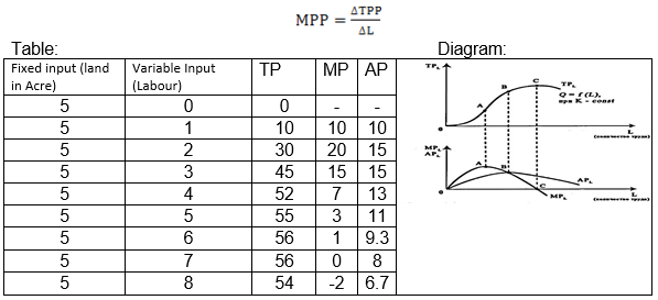
LAW OF VARIABLE PROPORTIONS: “Other things remaining constant when more and more variable inputs are employed with some fixed input , initially TP increase at increasing rate (MP increases) , then at diminishing rate (MP Declines) and at last declines (MP became negative).

Assumptions:

• There is at least one variable input and one fixed input (Operated in short run)

• Technique of production remain constant

Explanation:

This law can be explained with the help of the following table and Diagram

Explanation: This law can be explained through the following stages

  Stage-I: Increasing Returns to Factors (IRF)

• In this stage TP increase at increasing rate and MP increases

• This stage is called the stage of Increasing Returns to Factors (IRF) because the marginal product of the variable factor increases throughout this stage.

•  This stage ends at the point where the marginal product curve reaches its highest point.

• This is because the efficiency of the fixed factors increases as additional units of the variable factors are added to it

      Stage-II: (Diminishing Returns to Factors (DRF)

• In this stage, total product continues to increase but at a diminishing rate until it reaches its maximum point

• In this stage the marginal product of labour is diminishing but remains positive.

• This stage starts from the point where Mp curve starts declining and ends where MP is zero corresponds to the maximum point of TP curve

•  This is because the fixed factor becomes inadequate relative to the quantity of the variable factor

• This stage is important because the firm will seek to produce in this range.

      Stage- III :(Negative Returns to Factors (NRF)

• In this stage TP declines and MP became negative

• This stage starts from the point where MP became negative

• This is because the variable factor (labour) is too much relative to the fixed factor.

LAW OF DIMINISHING MARGINAL PRODUCT:

Law of diminishing marginal product Sometimes referred to as variable factor proportions, law of diminishing returns states that as equal quantities of one variable factor are increased, while other factor inputs remain constant, a point is reached beyond which the addition of one more unit of the variable factor will result in a diminishing rate of return and the marginal physical product will fall.

Explanation: The reason behind the law of diminishing returns or the law of variable proportion is the following.

• As we hold one factor input fixed and keep increasing the other, the factor proportions change.

• Initially, as we increase the amount of the variable input, the factor proportions become more and more suitable for the production and marginal product increases.

• But after a certain level of employment, the production process becomes too crowded with the variable input and the factor proportions become less and less suitable for the production.

This law can be explained through a table and diagram

(As in the above schedule and diagram of Law of Variable Proportions) 

Cost

Cost in economics is the expenditure incurred on factor and non-factor inputs of production.

Short Run Costs: -

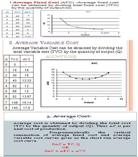
1.Total Fixed Cost- Fixed costs (also known as supplementary costs or overhead costs) are the costs that do not change with the level of output. Examples – Rent for factory building, interest, insurance premium, salaries of permanent employees, etc.

2.Total Variable Cost- Variable costs (or prime costs) are the costs that vary directly with the level of output. These are the expenses incurred on variable factor of production. Example- Expenses on raw materials, power and fuel, wages of casual workers, etc.

1.Total Cost –Total Cost in economics comprises of two elements: explicit cost and implicit cost. Actual money expenditure on inputs is termed as explicit cost. Estimated money value of inputs supplied by the owners of production unit, including normal profit, is termed as implicit cost. Main examples are: estimated salary of the owners, estimated interest of own money invested by the owners, estimated rent of the owner’s building, etc.  Thus in the short run TC is the sum total of TFC and TVC.

                TC = TFC + TVC

Unit Cost Curves in the Short Run

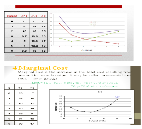
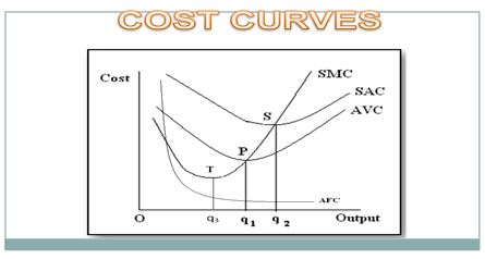
Important observations of AC, AVC & AFC

• AC curve always lie above AVC (because AC includes AVC & AFC at all levels of output).

• AVC reaches its minimum point at an output level lower than that of AC because when AVC is at its minimum AC is still falling because of fall in AFC.

• As output increases, the gap between AC and AVC curves decreases but they never intersect.

        Why is MC curve U shaped ?

The reason behind the U shape of the MC curve is the law of variable proportions. This implies that initially in the stage of increasing returns to a factor, marginal cost diminishes with the increase in the output, and then, after reaching a certain limit, in the stage of diminishing returns to a factor, marginal cost rises with further increases in the output. Thus the short run marginal cost curve becomes U shaped.

Why are AVC and AC curves U shaped ?

The shape of AVC and AC curves is influenced by the shape of MC curve in the short run. AVC and AC are U shaped because of operation of the law of variable proportion. Initially, in the stage of increasing returns when MC falls, the AVC and AC curves also falls. And after a certain level of output in the stage of diminishing returns when MC curve rises, the AVC and AC curves also rises. Thus, because of operation of law of variable proportion as output rises, the AVC and AC curves first fall, reach their minimum and then begin to rise. That is why AVC, AC and MC all are U shaped.

Important formulae at a glance

TFC = TC – TVC or TFC=AFC x output or

 TFC = TC at 0 output.

TVC = TC – TFC or TVC = AVC x output or

  TVC =∑MC

TC = TVC + TFC or TC = AC x output or

TC = ∑ MC + TFC

MC_n=TC_n – TC_n-1 or MC_n= TVC_n – TVC_n-1

AFC = TFC / Output or AFC = AC-AVC or

 ATC – AVC

AVC = TVC / Output or AVC = AC-AFC

AC = TC / Output or AC=AVC + AFC

REVENUE

MEANING:-Money received by a firm from the sale of a given output in the market.

TYPES OF REVENUE:-

Total Revenue: Total sale receipts or receipts from the sale of given output.

            TR    =      Quantity sold × Price     (or)     output sold × price

Average Revenue: Revenue or Receipt received per unit of output sold.

AR  = TR / Output  sold

AR and price are the same.

TR  =P x Q

AR   =  P x Q / Q

AR= price

AR and demand curve are the same. It shows the various quantities demanded at different prices. 

Marginal Revenue: Additional revenue earned by the seller by selling an additional unit of output.

 MR_n = TR _n -   TR _n-1              

MR  =   ∆ TR / ∆ Q       (OR)  TR = ∑ MR

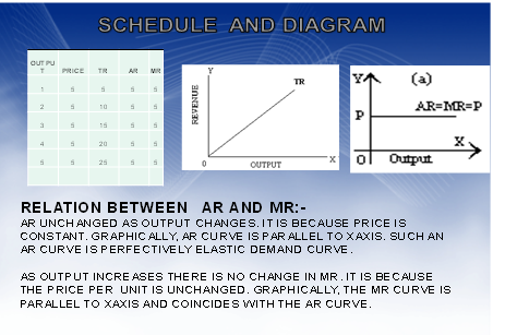
RELATION  BETWEEN TR AND MR

Under perfect competition, the sellers are price takers. Single price prevails in the market. Since all the goods are homogeneous and are sold at the same price AR = MR. As a result AR and MR curve will be horizontal straight line parallel to OX axis. (When price is constant or perfect competition)

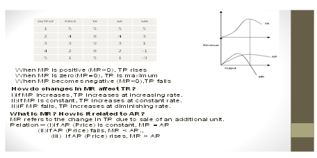
Relationship between AR and MR under monopoly and monopolistic competition (Price changes or under imperfect competition)

 AR and MR curves will be downward sloping in both the market forms.

• AR lies above MR.

• AR can never be negative.

• AR curve is less elastic in monopoly market form because of no substitutes.

• AR curve is more elastic in monopolistic market because of the presence of substitutes.

PRODUCER’S EQUILIBRIUM

CONTENT/ GIST OF THE CHAPTER

Definition:--A producer is said to be in equilibrium when he produces that level of output at which his profit is maximum .Producer’s equilibrium is also known as profit maximization situation.

Methods for determination of Producer’s Equilibrium.

1)   TR-TC  Approach

2)   MR –MC Approach

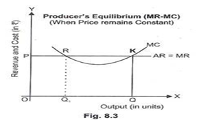
*Conditions of producer’s equilibrium under MR-MC approach when price is constant.(perfect competition) :

1)   MR=MC   2)  MC must be rising.

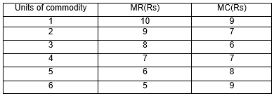
SITUATION ----1

According to table , both the conditions of equilibrium are satisfied at 4 units of output. MC =MR and MC rising.MC is more than MR when output is produced after 4 units of output. So producer’s equilibrium will be achieved at 4 units of output. However , MR =MC at 2 units of output also. But second condition is not fulfilled here. Let us understand Producer’s Equilibrium with the help of a diagram. Producer’s equilibrium is determined at OQ level of output corresponding to point k. As at this point MC=MR and MC cuts MR curve from below. When MR>MC at point R then producer will continue to produce as long as MR=MC , because firm will find it profitable to raise the output level. When MR< MC  above the point k then producer will cut down production as long as MR = MC ,because firm will find it unprofitable to produce an extra unit. So it

starts reducing the level of output till MR=MC.

Producer’s equilibrium when price falls with a rise in output under MR-MC approach is determined where (imperfect competition):

1)   MR=MC .2) MC must be rising.

SITUATION --2

When price falls with rise in output , MR curve slopes downward. Let us understand this with the help of following table.

According to the Table both the conditions of equilibrium are satisfied at 4 units of output. MC=MR and MC is rising.MC is more than MR when output is produced after 4 units of output. So producer’s equilibrium will be achieved at 4 units of output.

Let us understand the determination of equilibrium with the help of a diagram:In Figure output is shown in the X axis and revenue ,cost in the Y axis.

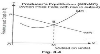
Producer’s Equilibrium is determined at OM level of output corresponding to the point E, where both the conditions are satisfied. When MR>MC  then producer will continue to produce  as long as MR=MC ,because firm will find it profitable to raise the output level.

When MR< MC  above the point E then producer will cut down production as long as MR = MC ,because firm will find it unprofitable to produce an extra unit. So it starts reducing the level of output till MR=MC. So the producer is at equilibrium at OM level of output.

                                                          SUPPLY

Meaning of supply;

Supply of a commodity by a firm or seller may be defined as the quantity of a commodity that a firm or seller offers for sale at a given price during a given time period.

Factors  determining  supply  or  determinants of supply of a good:-

(i)    Price of the commodity

(ii)   Price of other related good

(iii)  Price of inputs/factors

(iv)  Taxation policy of government

(v)   Objective of the firm

(i)    Price  of  the  commodity:  Other  factors  determining  supply  remaining constant, there is a direct relationship between price and quantity supplied of a commodity. It means the quantity supplied of a commodity increases with rise in price and decreases with fall in price of the commodity. Due to this direct relationship between price and quantity supplied of   a commodity the supply curve has a positive slope. Supply curve is upward sloping to the right.

(ii)   Price of other related goods: Supply of a commodity is also influenced by the change in the price of other related goods. With the help of given resources we can produce several goods by using the same technology. For example, a farmer can produce either pulses or food grains by using the resources. If the price of  pulses  increases  it  becomes  more  profitable  for  him  to  make  more production of pulses. So he will divert some resources from the production of food grains to the production of pulses. The production of pulses will increase and that of food grains will decrease. So the supply of pulses will increase if the price of pulses increases and the supply of food grain will decrease at the same price reverse will happen if the price of food grains increases.

(iii) Price of inputs/factors: Change in the price of input slike raw material, wage, rent or interest also influences the supply of a commodity. For example, in the production of cloth, cotton is the main raw material. If the price of cotton increases, the cost of production of cloth will increase. At the same price, the margin of profit will decrease. So the producer will decrease the supply of cloth at the same price. On the other hand if the price of cotton falls, the cost of production per unit of cloth will decrease and hence the supply of cloth will increase. The price of other inputs will also influence the supply of a good in the same manner.

(iv)Technology of production: An improvement in the technology of production of a commodity decreases the per unit cost of the commodity. The margin of profit will increase at the same price. So the supply of a commodity will increase, with improvement in technology of production, at the same price. On the other hand if a firm uses absolute technology of production, the cost of production per unit of the commodity will increase. The margin of profit will decrease, so the firm will decrease its supply at the same price. This is the main reason that the firms are trying to use better technology of production because it not only reduces the cost of production per unit but also improves the quality of the product.

(v) Taxation policy of government: If the government reduces the excise duty or the production of a commodity, the cost of production per unit of the commodity will decrease, the margin of profit will increase at the same price so the producer of the commodity will increase its supply. It happens when the government wants to increase the production of the commodity. On the other  hand  to  discourage  the  production  of  some  harmful  goods,  like cigarettes, liquor etc, the government increases the rate of excise duty on the production  of  such  goods.  So, the cost of  production  per  unit  of  the commodity increases and the supply of such commodities decreases.

(vi)  Objective of the firm: The objective of the producer also influences the supply of a commodity .Generally, the objective of a producer is to maximize his profits. Profits are maximized at a higher price. So he increases the supply of a commodity at a higher price and decreases its supply at a lower price. But sometimes,theproducermaybeinmaximizinghissalesandnotinmaximizing his  profits  as  he  wants  to  capture  the  market.  In that case, he  goes  on increasing the supply so long his target is not achieved. He may increase the supply at the same price to any extent.

SUPPLY FUNCTION

When the relationship between quantity supplied and the determinants of supply is expressed mathematically in an equation, it is called a supply function. So a supply function can be expressed as:

Sn = f(Pn, Pr, Pf, T, Tr, G)

where    Sn   =  Supply of commodity n

Pn  =  Price of the commodity n

Pr  =  Price of other related goods

Pf  =  Price of inputs/factors

T  =  Technology of production

Tr  =  Government policy or tax rate

G  =  Goal or objective of the producer

LAW OF SUPPLY

The law of supply depicts the relationship between price and quantity supplied of a commodity when all other determinants of supply remain constant. This law states that there is a direct relationship between price and quantity supplied of a commodity, other factors  determining  supply  remaining  constant.  It  means quantity supplied of a commodity increases with increase in price and decreases with decrease in price.

Individual and Market Supply

Individual Supply

Individual supply refers to the quantity of a commodity which an individual firm is willing to sell at a given price during a given period of time. It is related with the supply of an individual firm.

Table 19.1: Supply schedule of commodity x

Price (Rs.)                      Quantity supplied (units)

5                                                           0

6                                                           3

7                                                           6

8                                                           9

9                                                          12

Market Supply : Market supply is the collective supply of all the firms in the market of a commodity at different prices during a given period of time. Market supply can be derived by summing up the supply of all the individual firms in the market.

Supply Schedule :

Supply schedule is a table showing different quantities of a commodity that a firm is willing to sell at different prices during a given period of time. Supply schedule can be of two types.

(i)   Individual supply schedule: When we represent a single firm, willingness to sell different quantities of a commodity at different prices during a given time period, we get individual supply schedule.

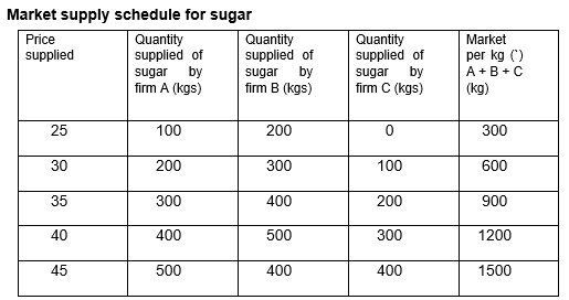
(ii)   Market  supply  schedule:  Market  supply  schedule  is  constructed  by summing up the supplies of all the individual firm at different prices during a given period of time. Amarket supply schedule is a table showing the total supply of a good by all the firms at different price during a given time period   Market  supply  schedule  can  be  explained  with  the  help  of  the following table.

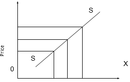
Supply Curve

Supply curve is the graphical presentation of a supply schedule. It shows the quantity that all the firms in the market are willing to supply at a given price during a given time period when all other factors influencing supply remain constant. Supply curve is also of two types.

Quantity supplied

(i)    Individual supply curve: Graphical presentation of individual supply schedule is called  individual  supply  curve.  It  shows  the  different  quantities  of  a commodity, an individual firm is willing to sell at different prices during a given time period.

(ii)   Market  supply  curve:  Market  supply  can  be  derived  by  horizontal summation of all individual supply curve: It show the different quantities of a commodity that all the firms are willing to sell at different prices during a given time period.

MOVEMENT ALONG SUPPLY CURVE AND SHIFT IN SUPPLY CURVE

All the factors determining supply of a commodity can be classified into two parts:----

I) Movement along supply curve due to change in the price of the commodity. In the law of supply, the quantity supplied of a commodity increases with increase in price and decrease with decrease in price all other determinants of supply remaining constant. These increase and decrease in supply are also termed as expansion and contraction of supply respectively .Expansion of supply is shown through an  upward  movement  along  the  same  supply  curve  on  the  other  hand contraction of supply is shown through downward movement on the same supply curve.

Movement along the supply curve or expansion and contraction of supply can be explained with the help of the following diagram.

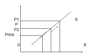
In  the  above  figure  initial  price  and  quantity  supplied  are  OP  and  OQ respectively. When the price increased from OP to OP1, the quantity supplied increases from OQ to OQ1. This is shown by upward movement from point A to point B on the same supply curve. This upward movement of the same supply curve shows the expansion of supply.

On the other hand when the price falls from OP to OP2, the quantity supplied decreases from OQ to OQ2. This is shown by downward movement from point A to point C on the same supply curve. This downward movement on the same supply curve shows the contraction of supply.

We can say that change in price of the commodity leads to change in quantity supplied of the commodity. It is shown by movement on the same supply curve. Increase in quantity supplied reflects expansion of supply and decrease in quantity supplied reflects contraction of supply.

(ii) Shift in supply curve due to other factors determining supply. When there is change in factors other than the price of the commodity then either more is supplied at the same price or less supplied at the same price. In such cases, the price of the commodity remains constant but there is a change in other factors like change in the price of inputs, change in technology of production, change in price of other related goods, change in taxation policy of the government etc.

For example, there is an improvement in the technology of production of the commodity in question. It leads to decrease in per unit of cost production of the commodity. The firm is willing to sell more quantity of the commodity at the same price. So the supply other commodity increases at the same price. This increase in supply is shown by rightward shift of supply curve.

On the other hand if the firm uses inferior technology of production, the cost of production per unit of the commodity increases. The firm is willing to sell less quantity at the same price. So the supply of the commodity decreases the same price. This decrease in supply is shown by left wards hift of the supply curve.

The above case so f increase and decrease in supply can be shown with the help of the following figures.

Main factors causing increase in supply or rightward shift of supply Curve

(i)       Fall in the price of other related goods

(ii)      Fall in the price of inptus/factors

(iii)     use of better technology in production

(iv)    Decrease in the rate of excise duty by government

(v)      If  the  objective  of  producer  changes  from  profit maximization  to  sales maximization Main factors causing decrease in supply or leftward shift of supply curve

(i)       Increase in the price of other related goods

(ii)      Rise in the price of inputs/factors

(iii)     use of inferior technology in production

(iv)    Increase in the rate of excise duty by the government

(v)      If the objective of the producer changes from soles maximization to profit maximization.

ELASTICITY OF SUPPLY

Elasticity of supply:-Price Elasticity of Supply measures the degree of responsiveness of change in Supply by change in price of the good. Law of Supply measures direction of relationship between price & Supply where as elasticity measures the proportional change in Supply by change in price. 

TYPES OF ELASTICITY OF SUPPLY:-

1) Perfectly Elastic Supply ( Ed = ∞):-When Supply of a commodity rises or falls to any extent without any change in price, the Supply for the commodity is said to be perfectly elastic. It is an imaginary situation.

lighly Elastic Supply ( Ed >1) :- When change in price leads to more proportional change in Supply, the Supply is said to be highly elastic. If the supply curve is extended to the left it will touch y axis.

2)  Unitary Elastic Supply ( Ed = 1) :- When Proportional Change in Supply is equal to proportional change in price, the Supply is said to be unitary elastic. If supply curve is extended towards left it will touch origin.

3) Inelastic Supply ( Ed< 1) :- When Proportional change in Supply is less than proportional change in price, the Supply is said to be inelastic Supply. If supply curve is extended towards left it will touch x axis.

4)  Perfectly Inelastic Supply ( Ed = 0):- When the Supply for the commodity does not change as a result of change in its price, Supply is said to be perfectly in elastic.

MEASURING ELASTICITY OF SUPPLY:- There are two methods of measuring elasticity of Supply:

i)     PERCENTAGE OR PROPORTIONATE METHOD:- elasticity of Supply is measured by the ratio of proportional change in Supply & proportional change in price. Symbolically,

The absolute value of elasticity of Supply ranges from zero to infinity.