CBSE Class 12 Physics Magnetic Effects of Electric Current Exam Notes

CBSE Class 12 Physics Magnetic Effects of Electric Current Exam Notes Please refer to the examination notes which you can use for preparing and revising for exams. These notes will help you to revise the concepts quickly and get good marks.

MAGNETIC EFFECTS OF ELECTRIC CURRENT

Magnetic Effects of Electric Current – exam notes

INTRODUCTION

Oersted in 1820, by observing the deflection of a compass needle brought near a current-carrying conductor, discovered that a current-carrying conductor produces a magnetic field in the space around it. This field is described by the vector \(\vec B\), called the magnetic induction, flux density or simply the field vector, with units Wb/m² or tesla. For a current-carrying conductor it is computed either with the help of the Biot–Savart law or with Ampere’s law.

The Biot–Savart law is the magnetic analogue of Coulomb’s law, while Ampere’s law is analogous to Gauss’s law.

BIOT–SAVART LAW

This law gives a method for calculating the magnetic induction at any point in space around a conductor carrying a current. If a small element of length \(dl\) of a long conductor carries a current \(I\), the magnetic induction \(d\vec B\) at a point P at a distance \(r\) is

\[d\vec B=\dfrac{\mu_0}{4\pi}\,\dfrac{I\,(d\vec l\times\vec r)}{r^3}\]

Here \(\vec r\) is the position vector of the point P from the centre of the element of length \(dl\). If \(\theta\) is the angle which OP makes with the length of the small element, the magnitude is

\[|d\vec B|=\dfrac{\mu_0}{4\pi}\,\dfrac{I\,dl\,(r\sin\theta)}{r^3}=\dfrac{\mu_0}{4\pi}\,\dfrac{I\,dl\sin\theta}{r^2}\qquad(\because\ |d\vec l\times\vec r|=dl\,r\sin\theta)\]

where \(\mu_0\) is the permeability of free space and \(\dfrac{\mu_0}{4\pi}=10^{-7}\) Wb/(A m).

The direction of \(d\vec B\) is perpendicular to the plane containing the current element \(d\vec l\) and the position vector \(\vec r\) which joins \(d\vec l\) to P. The total magnetic induction for the conductor is \(\vec B=\int d\vec B\). The unit of magnetic induction \(B\) is weber/metre² or tesla.

\[1\ \text{tesla}=1\ \text{weber/metre}^2=1\ \text{newton/(ampere metre)}\]

The magnetic intensity \(H\) at any point in the magnetic field is related to the magnetic induction by

\[H=\dfrac{B}{\mu}\quad\text{or}\quad B=\mu H\]

where \(\mu\) is the permeability of the medium. The unit of magnetic intensity \(H\) is ampere/metre.

Maxwell’s cork-screw rule: if a right-handed cork-screw is rotated so that its tip moves in the direction of flow of current through the conductor, then the direction of rotation of the head of the screw gives the direction of the magnetic lines of force.

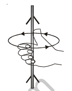
Right-hand rule: if the conductor is held in the right hand such that the thumb points in the direction of the current, the direction in which the fingers curl gives the direction of the magnetic field.

APPLICATIONS OF THE BIOT–SAVART LAW

1. Magnetic induction due to a long straight current-carrying conductor. Consider the current \(I\) flowing through a long conductor. If a small element CD of the conductor has length \(dl\), the field \(dB\) at P due to this element is given by the Biot–Savart law as

\[|d\vec B|=\dfrac{\mu_0}{4\pi}\dfrac{I\,dl\sin\theta}{x^2}\]

where \(x\) is the distance between the current element CD and the point P and \(\theta\) is the angle between CD and the line joining it with P. The total magnetic field is \(B=\int dB=\int\dfrac{\mu_0}{4\pi}\dfrac{I\,dl\sin\theta}{x^2}\).

If DE is perpendicular to CD, then in \(\Delta\)CDE, \(\sin\theta=\dfrac{DE}{CD}\), so \(dl=\dfrac{DE}{\sin\theta}\). Hence

\[B=\dfrac{\mu_0 I}{4\pi}\cdot\dfrac{DE}{\sin\theta}\cdot\dfrac{\sin\theta}{x^2}=\dfrac{\mu_0 I}{4\pi}\dfrac{DE}{x^2}\]

As \(\angle CPD=d\phi=\dfrac{DE}{x}\), we have \(DE=x\,d\phi\). Also in \(\Delta\)OPD, \(\dfrac{r}{x}=\cos\phi\), i.e. \(\dfrac1x=\dfrac{\cos\phi}{r}\). Therefore

\[B=\dfrac{\mu_0 I}{4\pi}\dfrac{x\,d\phi}{x^2}=\dfrac{\mu_0 I}{4\pi}\dfrac{\cos\phi\,d\phi}{r}\quad\Rightarrow\quad B=\dfrac{\mu_0 I}{4\pi r}\int\cos\phi\,d\phi\qquad\cdots(i)\]

The magnetic induction for different lengths of conductor can be found from equation (i):

1. Conductor of infinite length. When P lies opposite the middle point of the conductor, \(\phi\) varies from \(-\dfrac\pi2\) to \(\dfrac\pi2\): \(B=\dfrac{\mu_0I}{4\pi r}\displaystyle\int_{-\pi/2}^{\pi/2}\cos\phi\,d\phi=\dfrac{\mu_0 I}{2\pi r}\).
2. Conductor of finite length. If the conductor subtends an angle \(\phi_1\) above the line OP and \(\phi_2\) below OP at the point P: \(B=\dfrac{\mu_0I}{4\pi r}\displaystyle\int_{-\phi_2}^{\phi_1}\cos\phi\,d\phi=\dfrac{\mu_0I}{4\pi r}[\sin\phi]_{-\phi_2}^{\phi_1}=\dfrac{\mu_0I}{4\pi r}[\sin\phi_1+\sin\phi_2]\).
3. At the end of a conductor of infinite length. Here \(\phi_2=0\) and \(\phi_1=\dfrac\pi2\): \(B=\dfrac{\mu_0I}{4\pi r}\displaystyle\int_0^{\pi/2}\cos\phi\,d\phi=\dfrac{\mu_0I}{4\pi r}\).
4. At one end of a conductor of finite length. Here \(\phi_2=0\) and the other angle is \(\phi\): \(B=\dfrac{\mu_0I}{4\pi r}\displaystyle\int_0^{\phi}\cos\phi\,d\phi=\dfrac{\mu_0I\sin\phi}{4\pi r}\).
5. If P lies along the length of the conductor (on the line of the wire), \(B\) at P is zero.

2. Magnetic field on the axis of a current-carrying circular coil. If a current \(I\) flows in a circular coil of radius \(R\) and centre O, the field \(d\vec B\) due to an element AC of length \(dl\) on the circumference at a point P on the axis, at a distance \(r\) from the element, is given by the Biot–Savart law as

\[d\vec B=\dfrac{\mu_0}{4\pi}\dfrac{I\,(d\vec l\times\vec r)}{r^3}\]

The direction of \(dB\) at P is perpendicular to the line joining P to the element AC. As the angle between \(d\vec l\) and \(\vec r\) is 90°, \(dB\) can be resolved into two rectangular components: \(dB\cos\phi\) perpendicular to the axis and \(dB\sin\phi\) along the axis.

There is a symmetrical element A′C′ on the opposite part of the coil, which gives a field of equal magnitude at P. Its components perpendicular to the axis are equal in magnitude and opposite in direction, so they cancel for all such pairs of elements. The resultant field is therefore along the axis of the coil and is given by

\[|B|=\int dB\sin\phi=\dfrac{\mu_0}{4\pi}\dfrac{I}{r^2}\int dl\,\sin\phi\]

As \(\sin\phi=\dfrac Rr\), \(|B|=\dfrac{\mu_0 I R}{4\pi r^3}\int dl\), and with \(\int dl=2\pi R\):

\[B=\dfrac{\mu_0 I R\times2\pi R}{4\pi r^3}=\dfrac{\mu_0 I R^2}{2r^3}=\dfrac{\mu_0 I R^2}{2(R^2+x^2)^{3/2}}\]

If the coil has \(n\) turns,

\[|B|=\dfrac{\mu_0 nIR^2}{2(R^2+x^2)^{3/2}}\]

The field at the centre of the coil (\(x=0\)) is

\[B_0=\dfrac{\mu_0 nIR^2}{2R^3}=\dfrac{\mu_0 nI}{2R}\]

If the point P is at a very large distance from the coil, \(x\gg R\), then \(B_x=\dfrac{\mu_0nIR^2}{2x^3}\). If \(A=\pi R^2\) is the area of one turn,

\[B_x=\dfrac{\mu_0 nIA}{2\pi x^3}\]

A circular loop carrying current behaves like a magnetic dipole placed along the axis of the coil. If the current in one face appears to flow clockwise, that face behaves as a south pole; if the same face is seen from the opposite side, the current on it flows anticlockwise and it behaves as a north pole.

3. Magnetic field due to a circular arc. Consider a current \(I\) flowing through a circular arc of wire of radius \(r\). The field \(dB\) produced by the current through an element \(dl\) at the centre is, from the Biot–Savart law (the angle between \(d\vec l\) and \(\vec r\) is \(90^\circ\)),

\[|d\vec B|=\dfrac{\mu_0}{4\pi}\dfrac{I\,|d\vec l\times\vec r|}{r^3}=\dfrac{\mu_0}{4\pi}\dfrac{I\,dl\,r\sin 90^\circ}{r^3}=\dfrac{\mu_0 I\,dl}{4\pi r^2}\]

The magnetic induction due to the whole arc, with \(\int dl=r\phi\), is

\[B=\dfrac{\mu_0 I}{4\pi r^2}\int dl=\dfrac{\mu_0 I}{4\pi r^2}\times\phi r=\dfrac{\mu_0 I}{4\pi r}\,\phi\]

For a semicircular loop \(\phi=\pi\), so \(B=\dfrac{\mu_0 I}{4r}\).

The direction of \(\vec B\) for circular current-carrying conductors or closed loops: if the direction of the current coincides with the direction in which the fingers of the right hand curl, the stretched thumb points in the direction of the field inside the loop.

4. Magnetic field inside a current-carrying solenoid. A large number of turns of insulated wire wound in the form of a helix on a long cylindrical frame is called a solenoid. When a current is passed through it, a magnetic field is produced inside as well as outside the solenoid.

The Biot–Savart law can be used to calculate the field at any point on the axis. Let a current \(I\) flow in a solenoid having \(n\) turns per unit length. Consider an element AB of the coil of width \(dx\), located at a distance \(x\) from the point P where the field is to be found. The number of turns in the element is \(n\,dx\), so the field at P due to this elementary coil is

\[dB=\dfrac{\mu_0\,(n\,dx)\,I\,r^2}{2(r^2+x^2)^{3/2}}\]

where \(r\) is the radius of the solenoid. From the geometry, \(x=r\cot\theta\), so \(dx=-r\,\mathrm{cosec}^2\theta\,d\theta\). Then

\[dB=\dfrac{\mu_0\,N I r^2}{2(r^2+x^2)^{3/2}}\ \Rightarrow\ dB=\dfrac{\mu_0\,n I r^2\,(-r\,\mathrm{cosec}^2\theta\,d\theta)}{2\,(r^2+r^2\cot^2\theta)^{3/2}}\]

\[dB=-\dfrac{\mu_0 nIr^2\,\mathrm{cosec}^2\theta\,d\theta\cdot r}{2\,(r^2\,\mathrm{cosec}^2\theta)^{3/2}}=-\dfrac{\mu_0 nI\sin\theta\,d\theta}{2}\]

If the ends D and C of the solenoid subtend angles \(\theta_1\) and \(\theta_2\) at P with respect to the positive direction of the axis, the net field at P on the axis is

\[B=\int dB=-\dfrac{\mu_0nI}{2}\int_{\theta_1}^{\theta_2}\sin\theta\,d\theta=\dfrac{\mu_0nI}{2}\,[\cos\theta]_{\theta_1}^{\theta_2}\ \ \Rightarrow\ \ |B|=\dfrac{\mu_0nI}{2}\,[\cos\theta_1-\cos\theta_2]\]

1. If the solenoid is of infinite length, \(\theta_1=0\), \(\theta_2=180^\circ\): \(B=\dfrac{\mu_0nI}{2}[1-(-1)]=\mu_0nI\).
2. At the end of the last turn, \(\theta_1=90^\circ\), \(\theta_2=180^\circ\): \(B=\dfrac{\mu_0nI}{2}[0-(-1)]=\dfrac{\mu_0nI}{2}\).
3. At the end of the first turn, \(\theta_1=0\), \(\theta_2=90^\circ\): \(B=\dfrac{\mu_0nI}{2}[1-0]=\dfrac{\mu_0nI}{2}\).

FORCE ON A CHARGED PARTICLE IN A MAGNETIC FIELD

If a particle of charge \(q\) travels with a velocity \(\vec v\) in a uniform magnetic field \(\vec B\), it experiences a force \(\vec F\), called the Lorentz force, given by

\[\vec F=q(\vec v\times\vec B),\qquad |\vec F|=qvB\sin\theta\]

The direction of \(\vec F\) is perpendicular to both \(\vec v\) and \(\vec B\). Thus, if the magnetic field acts along the y-axis on a charge \(+q\) moving with velocity \(\vec v\) in the x–y plane making an angle \(\theta\) with the direction of \(\vec B\), the charged particle experiences a Lorentz force along the z-axis, which is mutually perpendicular to \(\vec B\) and \(\vec v\).

\[B=\dfrac{F}{qv\sin\theta}\]

If \(q=1\) coulomb, \(v=1\) m/s and \(\sin\theta=1\) (for \(\theta=90^\circ\)), then \(F=1\) newton, so \(B=1\) tesla \(=1\) weber/m².

Thus 1 tesla is the unit of magnetic field strength in SI units: it is the field which, acting on a charge of one coulomb moving with a velocity of 1 m/s at right angles to the field, deflects it with a force of 1 newton in a direction perpendicular to the field and the velocity. The CGS unit of magnetic induction is the gauss.

\[1\ \text{gauss}=1\ \text{oersted}=10^{-4}\ \text{tesla}\]

Trajectory of a charged particle in a magnetic field

1. If the velocity \(\vec v\) of the charged particle is parallel (\(\theta=0\)) or antiparallel (\(\theta=180^\circ\)) to \(\vec B\), then \(\vec F=0\) and the trajectory of the particle is a straight line.
2. If \(\vec v\) is perpendicular to \(\vec B\), i.e. \(\theta=90^\circ\), then \(F=Bqv\) and the direction of this maximum force is always perpendicular to \(\vec v\). The trajectory of the charged particle is a circular path.
3. If the particle makes an angle \(\theta\) with the field, where \(\theta\) lies between \(0^\circ\) and \(90^\circ\), the particle moves in a helix: the component \(v\sin\theta\), which is perpendicular to \(\vec B\), makes the charged particle move along a circle, whereas the component \(v\cos\theta\), which is parallel to \(\vec B\), makes it move along a straight line. The charged particle therefore moves along a helical path due to the superposition of the two motions.

If a particle of mass \(m\) and charge \(q\) moves in a magnetic field \(B\) with speed \(v\) in a circular path, the magnetic force provides the centripetal force:

\[Bqv=\dfrac{mv^2}{r}\quad\text{or}\quad\omega=\dfrac vr=\dfrac{Bq}{m}\]

\[\text{Frequency } f=\dfrac{Bq}{2\pi m},\qquad \text{time period } T=\dfrac{2\pi m}{Bq}\]

\(T\) is independent of \(v\).

If a particle with charge \(q\) moves with a speed \(\vec v\) where both an electric field \(\vec E\) and a magnetic field \(\vec B\) are present, the resultant force is

\[\vec F=q(\vec E+\vec v\times\vec B)\]

FORCE ON A CURRENT-CARRYING CONDUCTOR IN A MAGNETIC FIELD

Through experiments Ampere established that when a current element of length \(d\vec l\) is placed in a magnetic field \(\vec B\), it experiences a force

\[d\vec F=I\,d\vec l\times\vec B\]

where \(I\) is the current through the element. If \(d\vec l\) and \(\vec B\) are inclined at an angle \(\theta\) with each other, \(|d\vec F|=BI\,dl\sin\theta\). If \(\vec B\) is uniform over the length of the conductor,

\[\vec F=I(|\vec L\times\vec B|)\ \Rightarrow\ |\vec F|=BIL\sin\theta\]

where \(L\) is the length of the conductor. The direction of the force (given by Fleming’s left-hand rule) is always perpendicular to the plane containing the conductor and the magnetic field.

Fleming’s left-hand rule: if the left hand is stretched in such a manner that the thumb and the first two fingers of the left hand are mutually perpendicular to each other, and the first finger points in the direction of the field and the second (middle) finger in the direction of the current, then the direction of the thumb gives the direction of the force.

MAGNETIC FORCE BETWEEN TWO LONG PARALLEL CURRENT-CARRYING CONDUCTORS

Any current-carrying conductor produces a magnetic field around it. If another current-carrying conductor is placed near the first one, the second conductor experiences a force due to the magnetic field produced by the first conductor. Similarly, the first conductor experiences a force due to the magnetic field produced by the second. Thus both conductors exert force on each other due to the effects of their magnetic fields. The conductors attract each other if their currents are in the same direction, and they repel each other if their currents are in opposite directions.

Let two long parallel straight conductors P and Q be placed a distance \(r\) apart in the plane of the paper, carrying currents \(I_1\) and \(I_2\). The magnetic field \(B_1\) at Q due to conductor P is

\[B_1=\dfrac{\mu_0 I_1}{2\pi r}\]

The direction of \(\vec B_1\) is perpendicular to Q and perpendicular to the plane of the paper. The force acting per unit length of conductor Q is

\[F_2=\dfrac{\mu_0}{2\pi}\left(\dfrac{I_1I_2}{r}\right)\ \text{N/m}\]

Similarly, the force per unit length \(F_1\) on conductor P due to the current \(I_2\) is

\[F_1=\dfrac{\mu_0}{2\pi}\left(\dfrac{I_1I_2}{r}\right)\ \text{N/m}\]

Therefore the magnetic force between two parallel current-carrying conductors per unit length is

\[F=\dfrac{\mu_0}{2\pi}\left(\dfrac{I_1I_2}{r}\right)\ \text{N/m}\]

The force experienced by a length \(l\) of either conductor is \(\dfrac{\mu_0}{2\pi}\left(\dfrac{I_1I_2\,l}{r}\right)\).

If \(r=1\) m and \(I_1=I_2=1\) ampere, then \(F=2\times10^{-7}\) N.

Definition of the ampere: one ampere is that steady current which, when flowing through each of two infinitely long straight parallel wires placed 1 m apart in vacuum, produces a force of \(2\times10^{-7}\) N per metre of length on each wire.

EFFECT OF A MAGNETIC FIELD ON A CURRENT LOOP

Consider a rectangular loop PQRS having \(N\) turns, length \(l\), breadth \(b\) and area \(A\), placed in a uniform magnetic field \(\vec B\) in such a way that the normal to the coil subtends an angle \(\theta\) with the direction of \(\vec B\), when a current \(I\) flows through the loop clockwise.

The sides PQ and RS are perpendicular to the field, and equal and opposite forces of magnitude \(IlB\) act on them, upwards and downwards respectively. An equal and opposite force also acts on the sides QR and PS, towards the right and the left of the coil. The resultant force is zero but the resultant torque is not zero.

The forces on the sides PQ and RS produce a torque on a single turn, given by

\[\tau=IlbB\sin\theta=IAB\sin\theta\qquad(\because A=l\times b)\]

If there are \(N\) turns of similar loops in the coil,

\[\tau=NIAB\sin\theta=MB\sin\theta,\qquad\text{where }M=NIA\]

When \(\theta=0^\circ\), \(\tau=0\): the plane of the coil is perpendicular to the field. The torque is maximum when \(\theta=90^\circ\), i.e. when the plane of the coil is parallel to the field; then \(\tau=NIAB\).

Magnetic dipole moment. Comparing the above result with the torque experienced by a bar magnet of magnetic moment \(\vec M\) placed in a magnetic field \(\vec B\) (\(\vec\tau=\vec M\times\vec B\)), we conclude that a current-carrying loop behaves like a bar magnet of magnetic moment \(IA\), where \(\vec A\) is the area vector of the loop. For a current-carrying coil of \(N\) turns, the corresponding magnetic moment is \(NI\vec A\). The unit of magnetic moment is ampere metre².

The potential energy \(U\) of a magnetic dipole placed in a magnetic field is

\[U=-MB\cos\theta\quad\text{or}\quad U=-\vec M\cdot\vec B\]

The magnetic field \(\vec B\) at a large distance \(x\) on the axis of a dipole of magnetic moment \(M\) is

\[B=\dfrac{\mu_0}{4\pi}\left(\dfrac{2M}{x^3}\right)\]

The magnetic field \(\vec B\) at a large distance \(x\) on the equatorial line of a dipole of magnetic moment \(M\) is

\[B=\dfrac{\mu_0}{4\pi}\left(\dfrac{M}{x^3}\right)\]

Regarding the force on a current-carrying conductor in a magnetic field, some important points are given below:

1. As the force \(BI\,dl\sin\theta\) is not a function of position \(r\), the magnetic force on a current element is non-central (a central force is of the form \(\vec F=Kf(r)\hat n_r\)).
2. The force \(d\vec F\) is always perpendicular to both \(\vec B\) and \(I\,d\vec L\), though \(\vec B\) and \(I\,d\vec L\) may or may not be perpendicular to each other.
3. In the case of a current-carrying conductor in a magnetic field, the force acting is \(\vec F=\int I\,d\vec L\times\vec B=I\left[\int d\vec L\right]\times\vec B\) (if the magnetic field is uniform, i.e. \(B\) = constant). As for a conductor, \(\int d\vec L\) represents the vector sum of all the length elements from the initial to the final point, which by the law of vector addition is equal to the length vector \(\vec L'\) joining the initial and final points. So a current-carrying conductor of any arbitrary shape in a uniform field experiences a force \(\vec F=I\left[\int d\vec L\right]\times\vec B=I\vec L'\times\vec B\), where \(\vec L'\) is the length vector joining the initial and final points of the conductor.
4. If a current-carrying conductor in the form of a loop of any arbitrary shape is placed in a uniform field, \(\vec F=\oint I\,d\vec L\times\vec B=I\left[\oint d\vec L\right]\times\vec B\); for a closed loop the vector sum of the \(d\vec L\) is always zero. So \(\vec F=0\), i.e. the net magnetic force on a current loop in a uniform magnetic field is always zero. Here it must be kept in mind that in this situation different parts of the loop may experience elemental forces due to which the loop may be under tension, or may experience a torque. For a circular loop in a uniform field \(F=0\) and \(\tau=0\) (the loop is only under tension); for a rectangular loop with its plane parallel to the field \(F=0\) but \(\tau\ne0\).
5. If a current-carrying conductor is situated in a non-uniform field, its different elements experience different forces, so \(F_R\ne0\) but \(\tau\) may or may not be zero. If the conductor is free to move, it translates with or without rotation. For example, a loop in the field of a current-carrying wire AB has \(F_R\ne0\) and \(\tau=0\), while a current-carrying rod in the field of wire AB has \(F_R\ne0\) and \(\tau\ne0\).
6. If a current-carrying conductor in a magnetic field experiences a force and is free to move, work will be done and hence its kinetic energy will change, i.e. \(W=\Delta KE\) with \(W=\int\vec F\cdot d\vec s\). (Though \(\vec F=I(d\vec l\times\vec B)\), the real energy is supplied by the battery; the magnetic force does no work.)

MOVING COIL GALVANOMETER

It is based on the principle that when a current-carrying coil is placed in a uniform magnetic field, it experiences a force and a torque is produced which deflects the coil according to Fleming’s left-hand rule, and the current through the coil is proportional to the deflection of the coil. In a moving coil galvanometer the coil is suspended between the curved pole pieces of a horse-shoe type magnet. The pole pieces are made cylindrical and a soft iron cylindrical core is placed within the coil without touching it, which makes the field radial. In such a field the plane of the coil is always parallel to the field, such that the normal to the coil subtends an angle \(\theta\) equal to \(90^\circ\) with the direction of \(\vec B\). The torque deflecting the coil is given by

\[\tau=NBIA\]

As the coil deflects, a restoring torque is produced either in the suspension fibre or in the spring to which the pointer is attached. If \(\theta\) is the angle of twist, the restoring torque is \(\tau=C\theta\), where \(C\) is the restoring torque per unit twist. In the equilibrium position, \(NBIA=C\theta\), so

\[I=\left(\dfrac{C}{NBA}\right)\theta=K\theta\]

where \(\dfrac{C}{NBA}=K\) is a constant of the galvanometer. As the current is directly proportional to the deflection \(\theta\), the scale of the galvanometer can be calibrated to detect as well as measure small currents in milliamperes (mA) or microamperes (\(\mu\)A).

The current sensitivity of a galvanometer is the current required to produce unit deflection.

Conversion into an ammeter. A galvanometer G of resistance \(R_g\), capable of measuring a small current \(I_g\), can be converted into an ammeter capable of measuring a large current \(I\) by connecting a small resistance \(R_s\) in parallel with it, called the shunt resistance, such that

\[R_s=\dfrac{I_g}{I-I_g}\times R_g\]

Conversion into a voltmeter. Such a galvanometer can also be converted into a voltmeter of range \(V\) volts by connecting a high resistance \(R\) in series with it, whose value is given by

\[R=\dfrac{V}{I_g}-R_g\]