

Class 12 Physics Study Guide: CBSE Class 12 Physics Important Formulae All Chapters
Access comprehensive study materials and useful resources for Important Formulae using the CBSE Class 12 Physics Important Formulae All Chapters. Designed to align with the 2026-27 CBSE academic guidelines, these advanced resources help Class 12 Physics students reinforce core concepts beyond standard textbooks.
Download Important Formulae Study Material PDF
Access the complete useful resource PDF for Class 12 Physics below. Regular practice with these targeted academic notes builds familiarity with complex topics and helps secure higher marks in final school evaluations.
CBSE Class 12 Physics Important Formulae All Chapters. There are many more useful educational material which the students can download in pdf format and use them for studies. Study material like concept maps, important and sure shot question banks, quick to learn flash cards, flow charts, mind maps, teacher notes, important formulas, past examinations question bank, important concepts taught by teachers. Students can download these useful educational material free and use them to get better marks in examinations. Also refer to other worksheets for the same chapter and other subjects too. Use them for better understanding of the subjects.
IMPORTANT FORMULAE
IMPORTANT FORMULAE
1. ELECTROSTATICS
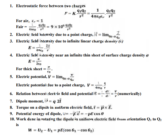
- Electrostatic force between two charges: \(F=K\dfrac{q_1q_2}{r^2}=\dfrac{1}{4\pi\epsilon_0\epsilon_r}\dfrac{q_1q_2}{r^2}\). For air, \(\epsilon_r=1\), so \(F_{air}=\dfrac{1}{4\pi\epsilon_0}\dfrac{q_1q_2}{r^2}=9\times10^9\dfrac{q_1q_2}{r^2}\).
- Electric field intensity due to a point charge: \(\vec E=\lim_{q_0\to0}\dfrac{\vec F}{q_0}\).
- Electric field intensity due to an infinite linear charge density (\(\lambda\)): \(E=\dfrac{1}{4\pi\epsilon_0}\cdot\dfrac{2\lambda}{r}\).
- Electric field intensity near an infinite thin sheet of surface charge density \(\sigma\): \(E=\dfrac{\sigma}{2\epsilon_0}\). For a thick (conducting) sheet, \(E=\dfrac{\sigma}{\epsilon_0}\).
- Electric potential, \(V=\lim_{q_0\to0}\dfrac{W}{q_0}\). Electric potential due to a point charge: \(V=\dfrac{1}{4\pi\epsilon_0}\cdot\dfrac qr\).
- Relation between electric field and potential: \(E=-\dfrac{dV}{dr}\ \left(=\dfrac Vr\text{ numerically, for a uniform field}\right)\).
- Dipole moment: \(\vec p=q\cdot2\vec l\).
- Torque on a dipole in a uniform electric field: \(\vec\tau=\vec p\times\vec E\).
- Potential energy of a dipole: \(U=-\vec p\cdot\vec E=-pE\cos\theta\).
- Work done in rotating the dipole in a uniform electric field from orientation \(\theta_1\) to \(\theta_2\): \(W=U_2-U_1=pE(\cos\theta_1-\cos\theta_2)\).
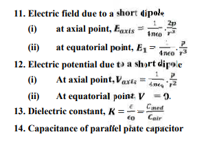
- Electric field due to a short dipole: (i) at an axial point, \(E_{axis}=\dfrac{1}{4\pi\epsilon_0}\cdot\dfrac{2p}{r^3}\); (ii) at an equatorial point, \(E_{eq}=\dfrac{1}{4\pi\epsilon_0}\cdot\dfrac{p}{r^3}\).
- Electric potential due to a short dipole: (i) at an axial point, \(V_{axis}=\dfrac{1}{4\pi\epsilon_0}\cdot\dfrac{p}{r^2}\); (ii) at an equatorial point, \(V=0\).
- Dielectric constant: \(K=\dfrac{\epsilon}{\epsilon_0}=\dfrac{C_{med}}{C_{air}}\).
- Capacitance of a parallel plate capacitor: (i) \(C=\dfrac{A\epsilon_0K}{d}\), in a medium of dielectric constant \(K\); (ii) \(C=\dfrac{A\epsilon_0}{d-t\left(1-\frac1K\right)}\), if the space between the plates is partially filled with a dielectric of thickness \(t\).
- Combination of capacitors: (i) in series, \(\dfrac1C=\dfrac1{C_1}+\dfrac1{C_2}+\dfrac1{C_3}\), \(q_1=q_2=q_3\), \(V=V_1+V_2+V_3\); (ii) in parallel, \(C=C_1+C_2+C_3\), \(q=q_1+q_2+q_3\), \(V_1=V_2=V_3=V\).
- Energy stored by a capacitor: \(U=\tfrac12CV^2=\dfrac{Q^2}{2C}=\tfrac12QV\).
- Electrostatic energy density: \(u_e=\tfrac12\epsilon_0E^2\) in air; \(u_e=\tfrac12\epsilon E^2\) in a medium.
- Total electric flux: \(\phi=\oint\vec E\cdot d\vec s=\dfrac{1}{\epsilon_0}\times\text{net charge enclosed by the surface}\).
2. CURRENT ELECTRICITY
- Electric current \(=\dfrac{\text{charge}}{\text{time}}\), i.e. \(I=\dfrac qt=\dfrac{ne}{t}\).
- For an electron revolving in a circle of radius \(r\) with speed \(v\): period of revolution \(T=\dfrac{2\pi r}{v}\); frequency of revolution \(\nu=\dfrac1T=\dfrac{v}{2\pi r}\); current \(I=e\nu=\dfrac{ev}{2\pi r}\).
- Ohm’s law: \(R=\dfrac VI\) or \(V=IR\).
- Current in terms of drift velocity (\(v_d\)): \(I=enAv_d\).
- Resistance of a uniform conductor: \(R=\rho\dfrac lA=\dfrac{ml}{ne^2\tau A}\).
- Resistivity or specific resistance: \(\rho=\dfrac{RA}{l}=\dfrac{m}{ne^2\tau}\).
- Conductance \(=\dfrac1R\).
- Conductivity \(=\dfrac1\rho\), or \(\sigma=\dfrac1\rho=\dfrac{l}{RA}\).
- Current density \(=\dfrac{\text{current}}{\text{area}}\), or \(j=\dfrac IA=env_d\).
- Relation between current density and electric field: \(j=\sigma E\) or \(E=\rho j\).
- Mobility: \(\mu=\dfrac{v_d}{E}\).
- Temperature coefficient of resistance: \(\alpha=\dfrac{R_2-R_1}{R_1(t_2-t_1)}\).
- The equivalent resistance \(R_s\) of a number of resistances connected in series is \(R_s=R_1+R_2+R_3+\ldots\)
- The equivalent resistance \(R_p\) of a number of resistances connected in parallel is given by \(\dfrac1{R_p}=\dfrac1{R_1}+\dfrac1{R_2}+\dfrac1{R_3}+\ldots\)
- EMF of a cell: \(E=\dfrac Wq\).
- For a cell of internal resistance \(r\), the emf is \(E=V+Ir=I(R+r)\).
- Terminal p.d. of a cell: \(V=IR=\dfrac{ER}{R+r}\).
- Terminal p.d. when a current is being drawn from the cell: \(V=E-Ir\).
- Terminal p.d. when the cell is being charged: \(V=E+Ir\).
- Internal resistance of a cell: \(r=R\left[\dfrac{E-V}{V}\right]\).
- For \(n\) cells in series: \(I=\dfrac{nE}{R+nr}\).
- For \(n\) cells in parallel: \(I=\dfrac{nE}{nR+r}\).
- Heat produced by an electric current: \(H=I^2Rt\) joule \(=\dfrac{I^2Rt}{4.18}\) cal.
- Electric power: \(P=\dfrac Wt=VI=I^2R=\dfrac{V^2}{R}\).
- Electric energy: \(W=Pt=VIt=I^2Rt\).
- Potential gradient of the potentiometer wire: \(k=\dfrac Vl\).
- For comparing the e.m.f.s of two cells: \(\dfrac{E_2}{E_1}=\dfrac{l_2}{l_1}\).
- For measuring the internal resistance of a cell: \(r=\dfrac{l_1-l_2}{l_2}\times R\).
- For a balanced Wheatstone bridge, \(\dfrac PQ=\dfrac RS\). If \(X\) is the unknown resistance, \(\dfrac PQ=\dfrac RX\) or \(X=\dfrac{RQ}{P}\).
- In a slide wire bridge, if the balance point is obtained at \(l\) cm from the zero end, then \(\dfrac PQ=\dfrac RX=\dfrac{l}{100-l}\).
3. MAGNETIC EFFECT OF CURRENT
- Biot–Savart law (magnetic field due to a current element): \(dB=\dfrac{\mu_0}{4\pi}\dfrac{I\,dl\sin\theta}{r^2}\).
- Force acting on a charge moving in a magnetic field: \(F=qvB\sin\theta\) or \(\vec F=q(\vec v\times\vec B)\).
- Magnetic field on the axis of a circular current loop: \(B=\dfrac{\mu_0NIa^2}{2(r^2+a^2)^{3/2}}\).
- Magnetic field due to an infinitely long straight current-carrying wire: \(B=\dfrac{\mu_0I}{2\pi r}\).
- Magnetic field at a point on the axis of a solenoid: \(B=\mu_0nI\).
- Motion of a charged particle in a uniform magnetic field: \(r=\dfrac{mv}{qB}\), \(T=\dfrac{2\pi m}{qB}\).
- Torque on a rectangular coil in a uniform magnetic field: \(\tau=NIBA\sin\theta\).
- Force per unit length acting on each of two straight parallel metallic conductors carrying current: \(f=\dfrac{F_2}{l}=\dfrac{\mu_0I_1I_2}{2\pi r}\).
- Deflection in a moving coil galvanometer: \(\alpha=\dfrac{NBAI}{k}\).
- Conversion of a galvanometer into an ammeter and a voltmeter: shunt \(S=\dfrac{I_gG}{I-I_g}\); series resistance \(R=\dfrac{V}{I_g}-R_G\).
- Elements of the Earth’s magnetic field: \(H=B_E\cos\theta\), \(V=B_E\sin\theta\).
- P.E. of a magnetic dipole in a uniform magnetic field: \(U=-mB\cos\theta\).
- Magnetic dipole moment of a revolving electron: \(m=\dfrac{evr}{2}=n\left(\dfrac{eh}{4\pi m_e}\right)\).
- Magnetising field intensity: \(H=nI\).
- Intensity of magnetization: \(M=\dfrac mV\).
4. ALL POSSIBLE FORMULAE AT A GLANCE — EMI AND AC
| Physical quantity | Formula | SI unit | Dimension |
|---|---|---|---|
| Magnetic flux (φ) | \(\vec B\cdot\vec A=BA\cos\theta=\int\vec B\cdot d\vec A\) | Wb = T m² | \([ML^2T^{-2}A^{-1}]\) |
| Induced emf (e) | \(\varepsilon=-\dfrac{d\phi}{dt}\). Induced current \(i=\dfrac{\varepsilon}{R}=-\dfrac NR\dfrac{d\phi}{dt}\). Induced charge \(q=i\Delta t=-\dfrac NR\Delta\phi\). Motional emf induced in a straight conductor: (i) linear motion \(=Blv\); (ii) rotation about one end \(=\dfrac{Bl^2\omega}{2}\) | Volt | \([ML^2T^{-1}A^{-1}]\) |
| Self-inductance | \(L=\dfrac{\phi}{I}\) and \(L=\dfrac{|\varepsilon|}{dI/dt}\). Self-inductance of a long solenoid: \(L=\mu_r\mu_0n^2Al\) | Henry | \([ML^2T^{-2}A^{-2}]\) |
| Mutual inductance | \(M_{12}=\dfrac{\phi_2}{I_1}\) and \(M_{12}=\dfrac{|\varepsilon_2|}{dI_1/dt}\). Mutual inductance of two long co-axial solenoids: \(M_{12}=\mu_0n_1n_2\pi r^2l\); \(M_{12}=\sqrt{L_1L_2}\) | Henry | \([ML^2T^{-2}A^{-2}]\) |
| Magnetostatic energy stored | \(U=\tfrac12LI^2\) | Joule | \([ML^2T^{-2}]\) |
| Alternating current and voltage | \(e=E_0\sin(\omega t+\phi)\) or \(e=E_0\cos(\omega t+\phi)\); \(i=I_0\sin(\omega t+\phi)\) or \(i=I_0\cos(\omega t+\phi)\). \(I_{rms}=I_0/\sqrt2=0.707I_0\) and \(E_{rms}=E_0/\sqrt2=0.707E_0\) | ||
| Phase relationship | For R: no phase difference between V and I. For L: voltage leads the current by \(\pi/2\). For C: current leads the voltage by \(\pi/2\). For an LCR circuit: if \(f>f_r\), \(\phi=\tan^{-1}\left(\dfrac{X_L-X_C}{R}\right)\) or \(\tan^{-1}\left(\dfrac{V_L-V_C}{V_R}\right)\); if \(f<f_r\), \(\phi=\tan^{-1}\left(\dfrac{X_C-X_L}{R}\right)\) or \(\tan^{-1}\left(\dfrac{V_C-V_L}{V_R}\right)\) | Unit less | Dimensionless |
| Reactance and impedance | Inductive reactance \(X_L=\omega L\); capacitive reactance \(X_C=1/\omega C\); impedance of an LR circuit \(Z=\sqrt{X_L^2+R^2}\); of an RC circuit \(Z=\sqrt{X_C^2+R^2}\); of an LCR circuit \(Z=\sqrt{(X_L-X_C)^2+R^2}\) | Ohm | \([ML^2T^{-1}A^{-2}]\) |
| Resonance frequency | \(f_r=\dfrac{1}{2\pi\sqrt{LC}}\), angular frequency \(\omega_r=\dfrac{1}{\sqrt{LC}}\) | Hertz, rad/s | \([T^{-1}]\) |
| Quality factor | \(Q=\dfrac1R\sqrt{\dfrac LC}=\dfrac{\omega_r}{2\Delta\omega}=\dfrac{\omega_rL}{R}=\dfrac{1}{\omega_rCR}\) | Unit less | Dimensionless |
| Power dissipated in an ac circuit | In a pure inductor and capacitor: zero. In a pure resistive circuit: \(I_0^2R/2\). In a combination of L, C and R: \(V_{rms}I_{rms}\cos\phi\) | Watt | \([ML^2T^{-3}]\) |
| Power factor | \(\cos\phi=R/Z\) | Unit less | Dimensionless |
| Wattless current | \(I_{rms}\cos\phi\) | Ampere | [A] |
| Frequency of LC oscillations | \(f_r=\dfrac{1}{2\pi\sqrt{LC}}\) | Hertz | \([T^{-1}]\) |
| Energy of an ideal LC oscillator | \(\tfrac12\dfrac{Q^2}{C}+\tfrac12LI^2=\tfrac12\dfrac{Q_0^2}{C}\) | Joule | \([ML^2T^{-2}]\) |
| Transformation ratio and efficiency | \(\dfrac{v_s}{v_p}=\dfrac{N_s}{N_p}\). Efficiency: \(\eta=\dfrac{v_sI_s}{v_pI_p}=\dfrac{P_o}{P_i}\) | Unit less | Dimensionless |
5. ELECTROMAGNETIC WAVES
- Speed of electromagnetic waves in vacuum: \(c=\dfrac{1}{\sqrt{\mu_0\epsilon_0}}=3\times10^8\) m/s.
- Ratio of the electric and magnetic field amplitudes: \(\dfrac{E_0}{B_0}=c\).
- Displacement current: \(I_D=\epsilon_0\dfrac{d\phi_E}{dt}\).
- Maxwell’s equations: (i) \(\oint\vec E\cdot d\vec A=\dfrac{Q}{\epsilon_0}\); (ii) \(\oint\vec B\cdot d\vec A=0\); (iii) \(\oint\vec E\cdot d\vec l=-\dfrac{d\phi_B}{dt}\); (iv) \(\oint\vec B\cdot d\vec l=\mu_0I+\mu_0\epsilon_0\dfrac{d\phi_E}{dt}\).
6. OPTICS
- Relation between focal length and radius of curvature of a mirror: \(f=R/2\).
- Mirror formula: \(\dfrac1f=\dfrac1v+\dfrac1u\).
- Magnification produced by a mirror: \(m=-\dfrac vu=-\dfrac{f}{u-f}\).
- Snell’s law: \(\dfrac{\sin i}{\sin r}={}_1n_2=\dfrac{n_2}{n_1}\); also \({}_2n_1=\dfrac{1}{{}_1n_2}\).
- \(n=\dfrac cv=\dfrac{\text{speed of light in vacuum}}{\text{speed of light in a medium}}=\dfrac{\lambda_{air}}{\lambda_{medium}}\).
- If the object is in a medium of refractive index \(n\), then \(n=\dfrac{\text{real depth}}{\text{apparent depth}}=\dfrac{t}{t_{app}}\).
- Apparent shift: \(x=t-\dfrac tn=t\left(1-\dfrac1n\right)\).
- Critical angle for total internal reflection: \(\sin C=\dfrac{1}{{}_an_d}=\dfrac1n\).
- Refraction at a spherical (convex) surface, for an object in the rarer medium and the real image in the denser medium: \(\dfrac{n_2}{v}-\dfrac{n_1}{u}=\dfrac{n_2-n_1}{R}\), where \(n_2\) and \(n_1\) are the refractive indices of the denser and rarer media.
- Lens formula: \(\dfrac1f=\dfrac1v-\dfrac1u\).
- Linear magnification produced by a lens: \(m=\dfrac IO=\dfrac vu\).
- Lens maker’s formula: \(\dfrac1f=\dfrac1v-\dfrac1u=({}_an_g-1)\left[\dfrac1{R_1}-\dfrac1{R_2}\right]=(n-1)\left[\dfrac1{R_1}-\dfrac1{R_2}\right]\).
- Power of a lens: \(P=\dfrac1f\) dioptre (\(f\) in metre).
- Lenses in contact: \(\dfrac1f=\dfrac1{f_1}+\dfrac1{f_2}\), or \(P=P_1+P_2\).
- Focal length of a lens in a liquid: \(f_l=\dfrac{{}_an_g-1}{\frac{{}_an_g}{{}_an_l}-1}\times f_a\).
- Refraction through a prism: \(r_1+r_2=A\) and \(i+e=A+\delta\), where \(A\) is the angle of the prism and \(\delta\) is the angle of deviation.
- For minimum deviation, \(i=e=i\) and \(r_1=r_2=r\). Therefore \(\delta_m=2i-A\).
- Refractive index of the material of the prism: \(n=\dfrac{\sin i}{\sin r}=\dfrac{\sin\left(\frac{A+\delta_m}{2}\right)}{\sin\left(\frac A2\right)}\).
- For a thin prism: \(\delta=(n-1)A\).
- Angular dispersion \(=\delta_V-\delta_R\).
- Dispersive power: \(\omega=\dfrac{\delta_V-\delta_R}{\delta_Y}=\dfrac{n_V-n_R}{n_Y-1}\).
- Simple microscope: magnifying power \(M=1+\dfrac Df\) (if the final image is at \(D\)); \(M=\dfrac Df\) (if the final image is at infinity).
- Compound microscope: (i) \(M=m_om_e\). (ii) For the final image at \(D\): \(M=-\dfrac{v_o}{u_o}\left\{1+\dfrac D{f_e}\right\}\approx-\dfrac L{f_o}\left\{1+\dfrac D{f_e}\right\}\). (iii) For the final image at infinity: \(M=-\dfrac{v_o}{u_o}\left\{\dfrac D{f_e}\right\}\approx-\dfrac L{f_o}\left\{\dfrac D{f_e}\right\}\).
- Astronomical telescope: (i) For the final image at infinity: \(M=-\dfrac{f_o}{f_e}\) and \(L=f_o+f_e\). (ii) For the final image at \(D\): \(M=-\dfrac{f_o}{f_e}\left\{1+\dfrac{f_e}{D}\right\}\) and \(L=f_o+u_e\).
- Resolving power. (i) For a microscope: the resolving power is the reciprocal of the limit of resolution, or separation between two points such that they are just distinct. R.P. \(=\dfrac1d=\dfrac{2n\sin\theta}{\lambda}\). Here \(d=\dfrac{\lambda}{2n\sin\theta}\) is the limit of resolution, \(n\sin\theta\) is the numerical aperture, and \(\theta\) is the well-resolved semi-angle of the cone of light rays of wavelength \(\lambda\) entering the microscope. (ii) For a telescope: the resolving power is the reciprocal of the angular limit of resolution, or angle subtended between two points such that they are just distinct. R.P. \(=\dfrac1{d\theta}=\dfrac{a}{1.22\lambda}\). Here \(d\theta=\dfrac{1.22\lambda}{a}\) is the angular limit of resolution, and \(a\) is the aperture or diameter of the objective lens.
- The distance for which ray optics is a good approximation for an aperture \(D\) and wavelength \(\lambda\) is called the Fresnel distance, given by \(Z_F=\dfrac{D^2}{\lambda}\).
Interference of light
- If two waves of the same intensity \(I_0\) interfere, then the resultant intensity will be \(I=4I_0\cos^2\dfrac\phi2\), where \(\phi\) is the initial phase difference between the waves.
- The resultant intensity at a point in the region of superposition is \(I=a_1^2+a_2^2+2a_1a_2\cos\phi=I_1+I_2+2\sqrt{I_1I_2}\cos\phi\), where \(I_1=a_1^2\) is the intensity of one wave and \(I_2=a_2^2\) is the intensity of the other wave.
- Condition for maxima: phase difference \(\phi=2n\pi\) and path difference \(=n\lambda\), where \(n=0,1,2,3,\ldots\)
- Condition for minima: phase difference \(\phi=(2n-1)\pi\) and path difference \(=(2n-1)\dfrac\lambda2\), where \(n=0,1,2,3,\ldots\)
- Fringe width \(\beta=\dfrac{D\lambda}{d}\), where \(D\) = distance between the slits and the screen, \(d\) = separation between the slits, and \(\lambda\) is the wavelength of light used.
- Angular fringe width \(\beta_\theta=\dfrac\beta D=\dfrac\lambda d\).
- Minimum amplitude \(A_{min}=(a_1-a_2)\).
- Minimum intensity \(I_{min}=(a_1-a_2)^2=I_1+I_2-2\sqrt{I_1I_2}\).
- Position of the \(n\)th maxima: \(y_n=\dfrac{nD\lambda}{d}\).
- Position of the \(n\)th minima: \(y_n=\left(n-\tfrac12\right)\dfrac{D\lambda}{d}\).
Diffraction of light
- The condition for the position of the \(n\)th minima: \(d\sin\theta=n\lambda\), where \(d\) is the width of the slit, \(\theta\) is the angle of diffraction and \(\lambda\) is the wavelength of light used.
- Linear half-width of the central maximum: \(y=\dfrac{D\lambda}{d}\).
- Total linear width of the central maximum: \(\beta_0\) or \(2y=\dfrac{2D\lambda}{d}\).
Polarization of light
- Brewster’s law: \(n=\tan i_p\).
- Malus’ law: \(I=I_0\cos^2\theta\).
7. ATOMS AND NUCLEI
Gist of lesson / formulae and shortcut formulae
- Rutherford’s α-particle scattering experiment (Geiger–Marsden experiment). Important observation: scattering of α-particles by heavy nuclei is in accordance with Coulomb’s law. Rutherford observed that the number of α-particles scattered is given by \(N\propto\dfrac{1}{\sin^4(\theta/2)}\).
- Distance of closest approach: estimation of the size of the nucleus. \(r_0=\dfrac{1}{4\pi\epsilon_0}\dfrac{Ze\times2e}{\frac12mv^2}\).
- Impact parameter (b). \(b=\dfrac{Ze^2\cot\frac\theta2}{4\pi\epsilon_0\left(\frac12mu^2\right)}\).
- Bohr’s atomic model. Radius of orbit: \(r=\dfrac{(4\pi\epsilon_0)n^2h^2}{4\pi^2mZe^2}\). Frequency: \(\nu=\dfrac{2\pi Ze^2}{(4\pi\epsilon_0)nh}\). Speed: \(v=\dfrac{2\pi Ze^2}{(4\pi\epsilon_0)ch}\times\dfrac{c}{n}=\alpha\dfrac{Zc}{n}\), where \(\alpha=\dfrac{2\pi e^2}{(4\pi\epsilon_0)ch}=\dfrac{1}{137}\) is called the fine structure constant.
- Energy of the electron. \(E_n=-\dfrac{mZ^2e^4}{8\epsilon_0^2h^2}\left(\dfrac1{n^2}\right)=-\dfrac{Z^2Rch}{n^2}\), where \(R=\dfrac{me^4}{8\epsilon_0^2ch^3}=1.097\times10^7\ \text{m}^{-1}\) is called the Rydberg constant. For hydrogen, \(E_n=-\dfrac{13.6}{n^2}\) eV. Also \(\bar\nu=R\left[\dfrac1{n_1^2}-\dfrac1{n_2^2}\right]\), where \(\bar\nu\) is called the wave number. Short-cut formula: K.E. \(=-\)(Total energy); P.E. \(=-2\) K.E.
- Spectral series of the hydrogen atom: Lyman series (ultraviolet), Balmer series (visible), Paschen, Brackett and Pfund series (infrared).
- Energy level diagram for the hydrogen atom. The energy of an electron in the \(n\)th orbit is given by \(E_n=-\dfrac{13.6}{n^2}\) eV.
In the energy level diagram, the transitions to n = 1 form the Lyman series (ultraviolet), to n = 2 the Balmer series (visible), to n = 3 the Paschen series (IR), to n = 4 the Brackett series (IR) and to n = 5 the Pfund series (IR). Energy levels: n = ∞: 0; n = 7: −0.28; n = 6: −0.38; n = 5: −0.54; n = 4: −0.85; n = 3: −1.51; n = 2: −3.4; n = 1: −13.6 eV.
- Bohr’s quantisation condition of angular momentum. Consider the motion of an electron in a circular orbit of radius \(r\) around the nucleus. According to the de Broglie hypothesis, this electron is also associated with wave character. Hence a circular orbit can be taken to be a stationary energy state only if it contains an integral number of de Broglie wavelengths, i.e. we must have \(2\pi r=n\lambda\). But \(\lambda=\dfrac{h}{mv}\), so \(2\pi r=n\dfrac h{mv}\), i.e. \(mvr=n\dfrac{h}{2\pi}\). This is the famous Bohr’s quantisation condition for angular momentum.
- Atomic mass unit (u). One atomic mass unit is defined as \(\tfrac1{12}\)th of the actual mass of a C-12 atom. \(1\ \text{u}=\tfrac1{12}\times\text{mass of a C-12 atom}=\tfrac1{12}\times1.992678\times10^{-26}\ \text{kg}=1.66\times10^{-27}\ \text{kg}\).
- Electron volt (eV). It is the energy acquired by an electron when it is accelerated through a potential difference of 1 volt. \(1\ \text{eV}=1.6\times10^{-19}\) J, and \(1\ \text{MeV}=1.6\times10^{-13}\) J.
- Relation between amu and MeV. \(1\ \text{u}=1.66\times10^{-27}\ \text{kg}\approx931\ \text{MeV}\).
- Nuclear density (\(\rho\)) \(=2.3\times10^{17}\ \text{kg/m}^3\). Obviously, nuclear density is independent of the mass number \(A\).
- Isotopes. Atoms of an element which have the same atomic number but different mass numbers are called isotopes. For example, hydrogen has three isotopes: \({}_1^1\text{H}\), \({}_1^2\text{H}\) and \({}_1^3\text{H}\).
- Isobars. Atoms having the same mass number but different atomic numbers are called isobars. For example, \({}_1^3\text{H}\) and \({}_2^3\text{He}\); \({}_{17}^{37}\text{Cl}\) and \({}_{16}^{37}\text{S}\); \({}_{20}^{40}\text{Ca}\) and \({}_{18}^{40}\text{Ar}\).
- Isotones. Nuclides having the same number of neutrons are called isotones. For example, \({}_{17}^{37}\text{Cl}\) and \({}_{19}^{39}\text{K}\); \({}_{80}^{198}\text{Hg}\) and \({}_{79}^{197}\text{Au}\).
- Isomers. These are nuclei having the same atomic number and the same mass number but existing in different energy states. For example, a nucleus in its ground state and the identical nucleus in a metastable excited state are isomers.
- Properties of nuclear forces. (i) Nuclear forces are very short-range attractive forces. (ii) Nuclear forces are charge independent. (iii) Nuclear forces are non-central forces. (iv) Nuclear forces do not obey the inverse square law.
- Nuclear force as a function of the separation between two nucleons. The graph of nuclear force against separation \(r\) shows strong repulsion at small separation, the force becomes zero at about 0.5 fermi, and beyond that it is attractive: attraction increases and then decreases.
- Potential energy of a pair of nucleons as a function of separation between two nucleons. The potential energy U (MeV) is positive and large at small r, falls to a minimum of about −100 MeV at r = r0, and then rises to zero at large r (r in fermi).
- Mass defect (\(\Delta m\)): \(\Delta m=[Zm_p+(A-Z)m_n]-M_N\).
- Packing fraction (P.F.). It is defined as the mass defect per nucleon, i.e. \(\text{P.F.}=\dfrac{\Delta m}{A}\). The nucleus is stable if P.F. > 1 and unstable if P.F. < 1.
- Binding energy (B.E.). The binding energy of a nucleus may be defined as the energy required to break up a nucleus into its constituent protons and neutrons and to separate them to such a large distance that they may not interact with each other. It is equivalent to the energy of the mass defect, i.e. \(\text{B.E.}=\Delta m\times c^2\), or \(\text{B.E.}=\left[\{Zm_p+(A-Z)m_n\}-M_N\right]\times c^2\).
- Binding energy per nucleon: B.E. per nucleon \(=\dfrac{\text{B.E.}}{A}\).
- Binding energy curve. (A graph of B.E. per nucleon against mass number.)
- Importance of the binding energy curve. This curve can be used to explain the phenomena of nuclear fission and fusion. (i) Nuclear fission: there is an overall gain in the binding energy per nucleon when we move from heavy to medium-range nuclei; hence energy is released. This indicates that energy can be released when a heavy nucleus is broken into small fragments. This is called nuclear fission. (ii) Nuclear fusion: similarly, there is an overall gain in the binding energy per nucleon when we move from lighter to medium-range nuclei; hence energy is released. This indicates that energy can be released when two lighter nuclei fuse together to form a heavy nucleus. This is called nuclear fusion.
- Radioactivity. The phenomenon of spontaneous and continuous disintegration of the nucleus of an atom of a heavy element on its own, with the emission of certain types of radiations, is called radioactivity.
- α-particles, β-particles and γ-rays. When the radiations emitted by a radioactive element are placed under an electric or magnetic field, the radiations split into three rays, classified as α-particles, β-particles and γ-rays.
- α-particles: An α-particle is the nucleus of helium, or a doubly ionised He atom. It is denoted by \({}_2^4\text{He}\). Charge on an α-particle \(=+2e=3.2\times10^{-19}\) C. Mass of an α-particle \(=6.645\times10^{-27}\) kg. β-particles: β-particles are fast-moving electrons, denoted by \({}_{-1}^{0}e\) or \({}_{-1}^{0}\beta\). Charge on a β-particle \(=-1.6\times10^{-19}\) C. Mass of a β-particle \(=9.1\times10^{-31}\) kg. γ-rays: γ-rays are electromagnetic waves of wavelength about 0.01 Å. They do not have any charge.
- Explanation of the process of α-decay. α-decay is a process in which an unstable nucleus transforms itself into a new nucleus by emitting an α-particle. For example, \({}_{92}^{238}\text{U}\to{}_{90}^{234}\text{Th}+{}_2^4\text{He}+Q\). In general, \({}_Z^A\text{X}\to{}_{Z-2}^{A-4}\text{Y}+{}_2^4\text{He}+Q\), where \(Q\) is the energy released in α-decay, shared by the daughter nucleus and the α-particle. During α-decay the ratio \(\dfrac np\) increases.
- Explanation of the process of β-decay. The process of spontaneous emission of an electron (e⁻) or a positron (e⁺) from a nucleus is called β-decay. For example, \({}_{15}^{32}\text{P}\to{}_{16}^{32}\text{S}+{}_{-1}^{0}e+\bar\nu\). In general, \({}_Z^A\text{X}\to{}_{Z+1}^{A}\text{Y}+{}_{-1}^{0}e+\bar\nu\) or \({}_Z^A\text{X}\to{}_{Z-1}^{A}\text{Y}+{}_{+1}^{0}e+\nu\). During β-decay the ratio \(\dfrac np\) decreases.
- Explanation of the process of γ-decay. The process of spontaneous emission of a γ-ray photon during the radioactive disintegration of a nucleus is called γ-decay. In general, \({}_Z^A\text{X}^*\to{}_Z^A\text{X}+\gamma\).
- Radioactive decay. The spontaneous emission of radiation from a radioactive element is called radioactive decay.
- Decay law. The number of nuclei disintegrating per second of a radioactive sample at any instant is directly proportional to the number of undecayed nuclei present in the sample at that instant, i.e. \(\dfrac{dN}{dt}\propto N\), which gives \(N=N_0e^{-\lambda t}\).
- Half-life period (T). The time interval in which one-half of the radioactive nuclei originally present in a radioactive sample disintegrate is called the half-life of that radioactive substance. The S.I. unit of half-life is the second.
- Relation between decay constant (λ) and half-life period (T): \(\lambda=\dfrac{0.6931}{T}\).
- Mean life (τ): \(\tau=\dfrac{T}{0.6931}\).
- Activity or decay rate (R): \(R=-\dfrac{dN}{dt}=\lambda N\); \(R=R_0e^{-\lambda t}\).
- Units of activity. (1) Becquerel (Bq): one becquerel is the decay rate of one disintegration per second, i.e. 1 Bq = 1 decay/sec. The S.I. unit of activity is the becquerel. (2) Curie (Ci): one curie is the decay rate of \(3.7\times10^{10}\) disintegrations per second, i.e. 1 curie = \(3.7\times10^{10}\) decays/sec. (3) Rutherford (Rd): one rutherford is the decay rate of \(10^6\) disintegrations per second, i.e. 1 rutherford = \(10^6\) decays/sec.
8. DUAL NATURE OF MATTER AND RADIATION
- Energy of a photon: \(E=h\nu=\dfrac{hc}{\lambda}\).
- Number of photons emitted per second: \(N=\dfrac PE\).
- Momentum of a photon: \(p=mc=\dfrac{h\nu}{c}=\dfrac h\lambda=\dfrac Ec\).
- Equivalent mass of a photon: \(m=\dfrac{h\nu}{c^2}=\dfrac E{c^2}=\dfrac{h}{c\lambda}\).
- Work function: \(W_0=h\nu_0=\dfrac{hc}{\lambda_0}\).
- Kinetic energy of a photoelectron is given by Einstein’s photoelectric equation: \(K_{max}=\tfrac12mv^2=h\nu-W_0=h(\nu-\nu_0)=hc\left(\dfrac1\lambda-\dfrac1{\lambda_0}\right)\).
- If \(V_0\) is the stopping potential, the maximum kinetic energy of the ejected photoelectron is \(K=\tfrac12mv_{max}^2=eV_0\).
- Kinetic energy of de Broglie waves: \(K=\tfrac12mv^2=\dfrac{p^2}{2m}\).
- Momentum of de Broglie waves: \(p=\sqrt{2mK}\).
- Wavelength of de Broglie waves: \(\lambda=\dfrac hp=\dfrac h{mv}=\dfrac h{\sqrt{2mK}}\).
- de Broglie wavelength of an electron beam accelerated through a potential difference of \(V\) volts: \(\lambda=\dfrac h{\sqrt{2meV}}=\dfrac{1.23}{\sqrt V}\ \text{nm}=\dfrac{12.27}{\sqrt V}\ \text{Å}\).
- de Broglie wavelength associated with gas molecules of mass \(m\) at temperature \(T\) kelvin: \(\lambda=\dfrac h{\sqrt{2mkT}}\), where \(k\) is Boltzmann’s constant.
- The value of \(hc=12400\) eV Å.
- The value of \(hc=1240\times10^{-9}\) eV m (i.e. \(hc/e=1240\times10^{-9}\) V m).
9. SEMICONDUCTOR DEVICES
Formulae of this unit:
- \(I=I_0\left[\exp\left(\dfrac{eV}{nk_BT}\right)-1\right]\).
- \(R=\dfrac{V_1-V_2}{I}\).
- \(I_E=I_C+I_B\).
- \(\alpha=\dfrac{I_C}{I_E}\).
- \(\beta=\dfrac{I_C}{I_B}\).
- \(\alpha=\dfrac{\beta}{1+\beta}\).
- \(\beta=\dfrac{\alpha}{1-\alpha}\).
- Input resistance: \(r_i=\left(\dfrac{\Delta V_{BE}}{\Delta I_B}\right)_{V_{CE}}\).
- Output resistance: \(r_o=\left(\dfrac{\Delta V_{CE}}{\Delta I_C}\right)_{I_B}\).
- Voltage gain: \(A_V=\beta\left(\dfrac{R_{out}}{R_{in}}\right)\).
- (a) OR operation: \(Y=A+B\). (b) AND operation: \(Y=A\cdot B\). (c) NOT operation: \(Y=\bar A\).
- Combination of gates: (a) a NAND gate is a combination of AND and NOT gates; (b) a NOR gate is a combination of NOT and OR gates; (c) an XOR gate is a combination of two NOT gates, two AND gates and one OR gate.
10. COMMUNICATION SYSTEMS
- Modulation factor: \(\mu=\dfrac{A_m}{A_c}\) or \(\mu=\dfrac{A_m}{A_c}\times100\%\).
- If \(A_{max}\) and \(A_{min}\) are the maximum and minimum amplitudes of the carrier wave, then \(\mu=\dfrac{A_{max}-A_{min}}{A_{max}+A_{min}}\times100\%\).
- Modulating voltage: \(m(t)=A_m\sin\omega_mt\).
- Carrier voltage: \(c(t)=A_c\sin\omega_ct\).
- Instantaneous voltage of an A.M. wave: \(c_m(t)=A_c(1+\mu\sin\omega_mt)\sin\omega_ct=A_c\sin\omega_ct-\dfrac{\mu A_c}{2}\cos(\omega_c+\omega_m)t+\dfrac{\mu A_c}{2}\cos(\omega_c-\omega_m)t\).
- Component frequencies of an A.M. wave: (a) carrier frequency \(=f_c\); (b) USB \(=f_c+f_m\); (c) LSB \(=f_c-f_m\).
- Bandwidth \(=(f_c+f_m)-(f_c-f_m)=2f_m\).
- Length of a dipole antenna: \(l=\dfrac\lambda2=\dfrac{c}{2\nu}\).
- Number of channels \(=\dfrac{\text{total bandwidth of the channel}}{\text{bandwidth needed per channel}}\).
- Critical frequency for sky wave propagation: \(f_c=9(N_{max})^{1/2}\).
- The range of TV transmission: \(d=\sqrt{2hR}\), where \(h\) = height of the antenna and \(R\) = radius of the Earth.
- Population covered \(=\) population density \(\times\) area.
- Maximum distance covered in LOS communication: \(d_M=d_T+d_R=\sqrt{2Rh_T}+\sqrt{2Rh_R}\).
Free study material for Physics
Physics Class 12 Exam Resources: Important Formulae
Quick Revision Material for Important Formulae
Access comprehensive study material for Important Formulae, including revision notes, concept maps, and high-probability questions. These resources are designed in alignment with the latest 2026 CBSE syllabus for Class 12 Physics to support effective exam preparation.
Expert Notes and Solved Exam Questions
Designed around the official curriculum, these study guides guarantee standard compliance. Reviewing step-by-step solutions clarifies complex sub-topics within Important Formulae and demystifies standard marking schemes for Physics evaluations.
Additional Study Resources for Class 12
For peak performance in upcoming evaluations, integrate official Physics sample papers directly into your study schedule. Follow up your revision by attempting online MCQ tests for Important Formulae to refine calculation speed and precision.
FAQs
Our advanced study package for Important Formulae includes detailed concepts, diagrams, Mind Maps, and explanation of complex topics to ensure Class 12 students learn as per syllabus for 2026 exams.
The Mind Maps provided for Important Formulae act as visual anchors which will help faster recall during high-pressure exams.
Yes, teachers use our Class 12 Physics resources for lesson planning as they are in simple language and have lot of solved examples.
Yes, You can download the complete, mobile-friendly PDF of the Physics Important Formulae advanced resources for free.
Yes, our subject matter experts have updated the Important Formulae material to align with the rationalized NCERT textbooks and have removed deleted topics and added new competency-based questions.