

Official CBSE Study Materials for Class 12 Physics
Review targeted academic resources with the CBSE Class 12 Physics Formula Booklet. Built according to official CBSE standards for the 2026-27 term, these downloadable Class 12 Physics study materials support effective daily practice and deeper conceptual understanding for Formula Booklet.
Advanced Resources for Physics
Access the complete useful resource PDF for Class 12 Physics below. Regular practice with these targeted academic notes builds familiarity with complex topics and helps secure higher marks in final school evaluations.


This Class 12 Physics short formula booklet gives all the important formulae of the CBSE syllabus in one place. It covers units and dimensions, kinematics and projectile motion, Newton's laws, friction, work, power and energy, circular motion, centre of mass, rigid body dynamics, simple harmonic motion, waves, heat and thermodynamics, electrostatics, current electricity, capacitance, alternating current, magnetism, electromagnetic induction, ray and wave optics, modern physics, gravitation, fluid mechanics and sound waves.
Topics Covered
1. Unit and Dimensions
2. Rectilinear Motion, Projectile Motion & Vectors, Relative Motion
3. Newton's Laws of Motion and Friction
4. Work, Power & Energy
5. Circular Motion
6. Centre of Mass and Rigid Body Dynamics
7. Simple Harmonic Motion and String Waves
8. Heat & Thermodynamics
9. Electrostatics, Current Electricity and Capacitance
10. Alternating Current
11. Magnetic Effect of Current and Electromagnetic Induction
12. Geometrical Optics and Wave Optics
13. Modern Physics
14. Gravitation
15. Fluid Mechanics & Properties of Matter
16. Sound Waves
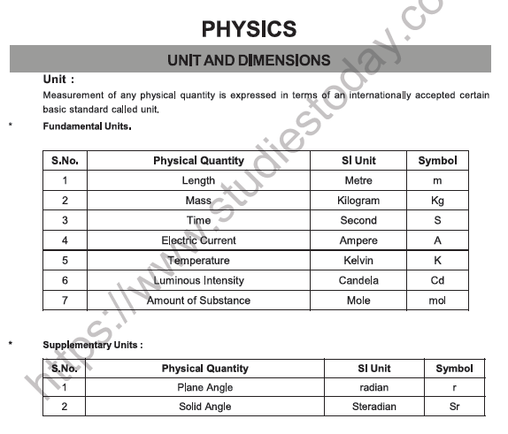
UNIT AND DIMENSIONS
Unit:
Measurement of any physical quantity is expressed in terms of an internationally accepted certain basic standard called unit.
Fundamental Units
| S.No. | Physical Quantity | SI Unit | Symbol |
|---|---|---|---|
| 1 | Length | Metre | m |
| 2 | Mass | Kilogram | kg |
| 3 | Time | Second | s |
| 4 | Electric Current | Ampere | A |
| 5 | Temperature | Kelvin | K |
| 6 | Luminous Intensity | Candela | cd |
| 7 | Amount of Substance | Mole | mol |
Supplementary Units
| S.No. | Physical Quantity | SI Unit | Symbol |
|---|---|---|---|
| 1 | Plane Angle | radian | rad |
| 2 | Solid Angle | Steradian | sr |
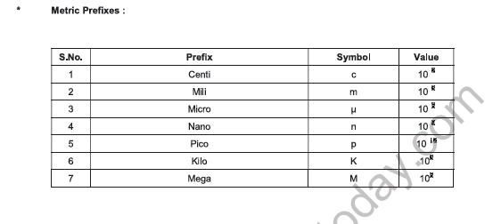
Metric Prefixes
| S.No. | Prefix | Symbol | Value |
|---|---|---|---|
| 1 | Centi | c | 10⁻² |
| 2 | Milli | m | 10⁻³ |
| 3 | Micro | μ | 10⁻⁶ |
| 4 | Nano | n | 10⁻⁹ |
| 5 | Pico | p | 10⁻¹² |
| 6 | Kilo | k | 10³ |
| 7 | Mega | M | 10⁶ |
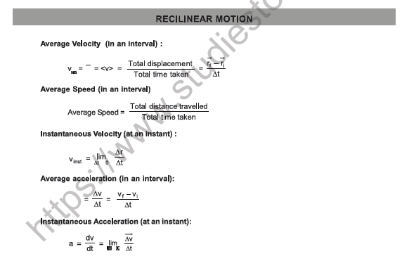
RECTILINEAR MOTION
Average Velocity (in an interval):
vav = ⟨v⟩ = \( \frac{\text{Total displacement}}{\text{Total time taken}} \) = \( \frac{\vec{r}_f - \vec{r}_i}{\Delta t} \)
Average Speed (in an interval):
Average Speed = \( \frac{\text{Total distance travelled}}{\text{Total time taken}} \)
Instantaneous Velocity (at an instant):
vinst = limΔt→0 \( \frac{\Delta \vec{r}}{\Delta t} \)
Average acceleration (in an interval):
aav = \( \frac{\Delta \vec{v}}{\Delta t} \) = \( \frac{\vec{v}_f - \vec{v}_i}{\Delta t} \)
Instantaneous Acceleration (at an instant):
a = \( \frac{dv}{dt} \) = limΔt→0 \( \frac{\Delta \vec{v}}{\Delta t} \)
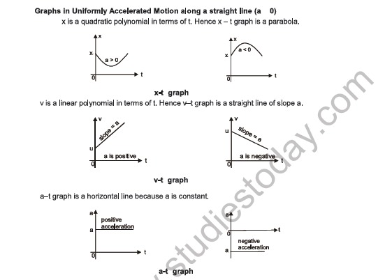
Graphs in Uniformly Accelerated Motion along a straight line (a ≠ 0)
x is a quadratic polynomial in terms of t. Hence x - t graph is a parabola.
[Figure: x-t graph - two parabolas on axes x (vertical) and t (horizontal), intercept x₀ on the x-axis; left curve opens upward, labelled a > 0; right curve opens downward, labelled a < 0]
v is a linear polynomial in terms of t. Hence v - t graph is a straight line of slope a.
[Figure: v-t graph - two straight lines starting from intercept u on the v-axis; left line rising, slope = a, labelled a is positive; right line falling, slope = a, labelled a is negative]
a - t graph is a horizontal line because a is constant.
[Figure: a-t graph - horizontal line at value a above the t-axis labelled positive acceleration; horizontal line at value a below the t-axis labelled negative acceleration]
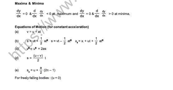
Maxima & Minima:
\( \frac{dy}{dx} \) = 0 and \( \frac{d}{dx}\left(\frac{dy}{dx}\right) \) < 0 at maximum, and \( \frac{dy}{dx} \) = 0 and \( \frac{d}{dx}\left(\frac{dy}{dx}\right) \) > 0 at minima.
Equations of Motion (for constant acceleration)
(a) v = u + at
(b) s = ut + \( \frac{1}{2} \)at², s = vt - \( \frac{1}{2} \)at², xf = xi + ut + \( \frac{1}{2} \)at²
(c) v² = u² + 2as
(d) s = \( \frac{u + v}{2} \) t
(e) sn = u + \( \frac{a}{2} \)(2n - 1)
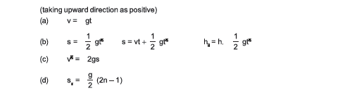
For freely falling bodies: (u = 0)
(taking upward direction as positive)
(a) v = gt
(b) s = \( \frac{1}{2} \)gt², s = vt + \( \frac{1}{2} \)gt², hn = h = \( \frac{1}{2} \)gt²
(c) v² = 2gs
(d) sn = \( \frac{g}{2} \)(2n - 1)
PROJECTILE MOTION & VECTORS
Time of flight: T = \( \frac{2u\sin\theta}{g} \)
Horizontal range: R = \( \frac{u^2 \sin 2\theta}{g} \)
Maximum height: H = \( \frac{u^2 \sin^2\theta}{2g} \)
Trajectory equation (equation of path):
y = x tan θ - \( \frac{gx^2}{2u^2\cos^2\theta} \) = x tan θ \( \left(1 - \frac{x}{R}\right) \)
Projection on an inclined plane
[Figure: A projectile launched from a point on an incline of angle β with the horizontal, at angle α to the incline; axes x along the incline (downward, towards the lower left) and y perpendicular to the incline]
| Up the Incline | Down the Incline | |
|---|---|---|
| Range | \( \frac{2u^2 \sin\alpha \cos(\alpha + \beta)}{g\cos^2\beta} \) | \( \frac{2u^2 \sin\alpha \cos(\alpha - \beta)}{g\cos^2\beta} \) |
| Time of flight | \( \frac{2u\sin\alpha}{g\cos\beta} \) | \( \frac{2u\sin\alpha}{g\cos\beta} \) |
| Angle of projection with incline plane for maximum range | \( \frac{\pi}{4} - \frac{\beta}{2} \) | \( \frac{\pi}{4} + \frac{\beta}{2} \) |
| Maximum Range | \( \frac{u^2}{g(1 + \sin\beta)} \) | \( \frac{u^2}{g(1 - \sin\beta)} \) |
RELATIVE MOTION
vAB (velocity of A with respect to B) = vA - vB
aAB (acceleration of A with respect to B) = aA - aB
Relative motion along straight line: xAB = xB - xA
CROSSING RIVER
A boat or man in a river always moves in the direction of resultant velocity of velocity of boat (or man) and velocity of river flow.
1. Shortest Time:
Velocity along the river, vx = vR
Velocity perpendicular to the river, vy = vmR
The net speed is given by vm = \( \sqrt{v_{mR}^2 + v_R^2} \)
[Figure: River of width d with banks as two horizontal lines; man starts at A on the lower bank, heads straight across (velocity vmR, perpendicular to the banks) while the river flows with vr; the resultant vm carries him along the dashed line to C on the opposite bank, drift = x from the point B directly opposite A; axes x along the river and y across]
2. Shortest Path:
Velocity along the river, vx = 0
and velocity perpendicular to river vy = \( \sqrt{v_{mR}^2 - v_R^2} \)
The net speed is given by vm = \( \sqrt{v_{mR}^2 - v_R^2} \) at an angle of 90° with the river direction.
Velocity vy is used only to cross the river, therefore time to cross the river, t = \( \frac{d}{v_y} \) = \( \frac{d}{\sqrt{v_{mR}^2 - v_R^2}} \)
and velocity vx is zero, therefore, in this case the drift should be zero.
vR - vmR sin θ = 0 or vR = vmR sin θ
or θ = sin⁻¹ \( \frac{v_R}{v_{mR}} \)
[Figure: River of width d; man starts at A on the lower bank and reaches B directly opposite on the upper bank; vmR is directed upstream at angle θ to the perpendicular, vr is the river velocity and vm the resultant, along AB; axes x along the river and y across]
RAIN PROBLEMS
vRm = vR - vm or vRm = \( \sqrt{v_R^2 + v_m^2} \)
NEWTON'S LAWS OF MOTION
1. From third law of motion
FAB = -FBA (vectors)
FAB = Force on A due to B
FBA = Force on B due to A
2. From second law of motion
Fx = \( \frac{dP_x}{dt} \) = max, Fy = \( \frac{dP_y}{dt} \) = may, Fz = \( \frac{dP_z}{dt} \) = maz
5. WEIGHING MACHINE:
A weighing machine does not measure the weight but measures the force exerted by object on its upper surface.
6. SPRING FORCE: F = -kx
x is displacement of the free end from its natural length or deformation of the spring where k = spring constant.
7. SPRING PROPERTY: k ℓ = constant
ℓ = Natural length of spring.
8. If spring is cut into two in the ratio m : n then spring constant is given by
ℓ1 = \( \frac{m\ell}{m+n} \); ℓ2 = \( \frac{n\ell}{m+n} \); kℓ = k1ℓ1 = k2ℓ2
For series combination of springs: \( \frac{1}{k_{eq}} \) = \( \frac{1}{k_1} \) + \( \frac{1}{k_2} \) + .......
For parallel combination of springs: keq = k1 + k2 + k3 ............
9. SPRING BALANCE:
It does not measure the weight. It measures the force exerted by the object at the hook.
Remember:
vP = \( \frac{V_1 + V_2}{2} \)
aP = \( \frac{a_1 + a_2}{2} \)
[Figure: Pulley system hanging from a fixed support; a block hangs over a fixed pulley, and a movable pulley P (moving with velocity vP) is supported by the string, with two blocks having velocities V1 and V2 hanging from it]
11. a = \( \frac{(m_2 - m_1)g}{m_1 + m_2} \)
T = \( \frac{2m_1 m_2 g}{m_1 + m_2} \)
[Figure: Atwood machine - a string over a fixed pulley with mass m1 moving up with acceleration a and mass m2 moving down with acceleration a, tension T on each side]
12. WEDGE CONSTRAINT:
[Figure: A block on the inclined face (angle θ) of a wedge that moves horizontally with velocity V1; the block has velocity V2 and its component perpendicular to the incline is V3, with V3 = V1 sin θ. Second sketch shows the contact plane at angle θ with component V1 sin θ]
Components of velocity along perpendicular direction to the contact plane of the two objects is always equal if there is no deformations and they remain in contact.
13. NEWTON'S LAW FOR A SYSTEM
Fext = m1a1 + m2a2 + m3a3 + ......
Fext = Net external force on the system.
m1, m2, m3 are the masses of the objects of the system and a1, a2, a3 are the acceleration of the objects respectively.
14. NEWTON'S LAW FOR NON INERTIAL FRAME:
Freal + Fpseudo = ma
Net sum of real and pseudo force is taken in the resultant force.
a = Acceleration of the particle in the non inertial frame
Fpseudo = -m aframe
(a) Inertial reference frame: Frame of reference moving with constant velocity.
(b) Non-inertial reference frame: A frame of reference moving with non-zero acceleration.
FRICTION
Friction force is of two types.
(a) Kinetic (b) Static
KINETIC FRICTION: fk = μk N
The proportionality constant μk is called the coefficient of kinetic friction and its value depends on the nature of the two surfaces in contact.
STATIC FRICTION:
It exists between the two surfaces when there is tendency of relative motion but no relative motion along the two contact surfaces.
This means static friction is a variable and self adjusting force. However it has a maximum value called limiting friction.
fmax = μs N
0 ≤ fs ≤ fsmax
[Figure: Block M on a rough surface (coefficients μs, μk) pulled by effort F towards the right, with friction f acting to the left. Graph of friction (vertical) against applied force (horizontal): a straight rising line labelled static friction up to the limiting value μsN, then a drop to a flat line at the kinetic value μkN]
WORK, POWER & ENERGY
WORK DONE BY CONSTANT FORCE: W = F · S (vectors)
WORK DONE BY MULTIPLE FORCES
ΣF = F1 + F2 + F3 + .....
W = [ΣF] · S ...(i)
W = F1 · S + F2 · S + F3 · S + ....
or W = W1 + W2 + W3 + ..........
WORK DONE BY A VARIABLE FORCE
dW = F · ds (vectors)
RELATION BETWEEN MOMENTUM AND KINETIC ENERGY
K = \( \frac{p^2}{2m} \) and P = \( \sqrt{2mK} \); P = linear momentum
POTENTIAL ENERGY
\( \int_{U_i}^{U_f} dU = -\int_{r_i}^{r_f} \vec{F} \cdot d\vec{r} \), i.e., U2 - U1 = -\( \int_{r_1}^{r_2} \vec{F} \cdot d\vec{r} \) = -W
U = -\( \int_{\infty}^{r} \vec{F} \cdot d\vec{r} \) = -W
CONSERVATIVE FORCES
F = -\( \frac{dU}{dr} \)
WORK-ENERGY THEOREM
WC + WNC + WP = ΔK
Modified Form of Work-Energy Theorem
WC = -ΔU
WNC + WP = ΔK + ΔU
WNC + WP = ΔE
POWER
The average power (P̄ or Pav) delivered by an agent is given by P̄ or Pav = \( \frac{W}{t} \)
P = \( \frac{F\,dS}{dt} \) = F \( \frac{dS}{dt} \) = F · v (vectors)
CIRCULAR MOTION
1. Average angular velocity
ωav = \( \frac{\theta_2 - \theta_1}{t_2 - t_1} \) = \( \frac{\Delta\theta}{\Delta t} \)
2. Instantaneous angular velocity
ω = \( \frac{d\theta}{dt} \)
3. Average angular acceleration
αav = \( \frac{\omega_2 - \omega_1}{t_2 - t_1} \) = \( \frac{\Delta\omega}{\Delta t} \)
4. Instantaneous angular acceleration
α = \( \frac{d\omega}{dt} \) = ω \( \frac{d\omega}{d\theta} \)
5. Relation between speed and angular velocity
v = rω and v = ω × r (vectors)
7. Tangential acceleration (rate of change of speed)
at = \( \frac{dV}{dt} \) = r \( \frac{d\omega}{dt} \) = ω \( \frac{dr}{dt} \)
8. Radial or normal or centripetal acceleration
ar = \( \frac{v^2}{r} \) = ω²r
9. Total acceleration
a = at + ar (vectors), a = \( \sqrt{a_t^2 + a_r^2} \)
Where at = α × r and ar = ω × v (vectors)
[Figure: Circular path with centre O; at point P the tangential acceleration at and velocity v point along the tangent, the radial acceleration ar (or ac) points towards O, and the total acceleration a lies between them at angle θ]
10. Angular acceleration
α = \( \frac{d\omega}{dt} \) (Non-uniform circular motion)
[Figure: Circular ring with ACW (anticlockwise) rotation; the angular acceleration α is shown as a vector perpendicular to the plane of the ring]
12. Radius of curvature R = \( \frac{v^2}{a_\perp} \) = \( \frac{mv^2}{F_\perp} \)
If y is a function of x, i.e. y = f(x):
R = \( \frac{\left[1 + \left(\frac{dy}{dx}\right)^2\right]^{3/2}}{\left|\frac{d^2y}{dx^2}\right|} \)
13. Normal reaction of road on a concave bridge
N = mg cos θ + \( \frac{mv^2}{r} \)
[Figure: Car moving with velocity V on a concave bridge; centre O above, angle θ between the vertical through O and the radius to the car; forces N along the radius towards O, mg downward and its component mg cos θ along the radius]
14. Normal reaction on a convex bridge
N = mg cos θ - \( \frac{mv^2}{r} \)
[Figure: Car moving with velocity V on a convex bridge; centre O below, angle θ at O; forces N outward along the radius, mg downward and its component mg cos θ along the radius]
15. Skidding of vehicle on a level road
vmax = \( \sqrt{\mu g r} \)
16. Skidding of an object on a rotating platform
ωmax = \( \sqrt{\mu g / r} \)
17. Bending of cyclist
tan θ = \( \frac{v^2}{rg} \)
18. Banking of road without friction
tan θ = \( \frac{v^2}{rg} \)
19. Banking of road with friction
\( \frac{v^2}{rg} \) = \( \frac{\mu + \tan\theta}{1 - \mu\tan\theta} \)
20. Maximum also minimum safe speed on a banked frictional road
vmax = \( \left[\frac{rg(\mu + \tan\theta)}{1 - \mu\tan\theta}\right]^{1/2} \)
vmin = \( \left[\frac{rg(\tan\theta - \mu)}{1 + \mu\tan\theta}\right]^{1/2} \)
21. Centrifugal force (pseudo force)
f = mω²r, acts outwards when the particle itself is taken as a frame.
22. Effect of earth's rotation on apparent weight
N = mg - mRω² cos² θ ; where θ = latitude at a place
23. Various quantities for a critical condition in a vertical loop at different positions (True for a string or on a smooth track.)
[Figure: Circle with centre O, points A (bottom), B (right), C (top) and D (left), and a particle at P at angle θ with normal N]
(1), (2) and (3) are three set-ups of a body on a string or moving inside a smooth track (circular loop or a ring track).
vmin at the lowest point = \( \sqrt{5gL} \) (for completing the circle) in each of the three cases.
24. Conical pendulum:
T cos θ = mg
T sin θ = mω²r
Time period = 2π \( \sqrt{\frac{L\cos\theta}{g}} \)
[Figure: Conical pendulum - a bob of mass mg on a string of length L from a fixed point of suspension, string at angle θ to the vertical, tension T with components T cos θ (vertical) and T sin θ (horizontal), moving in a horizontal circle of radius r at depth h below the suspension]
25. Relations among angular variables:
ω0 = Initial angular velocity
ω = Final angular velocity
α = Constant angular acceleration
ω = ω0 + αt
θ = ω0t + \( \frac{1}{2} \)αt²
ω² = ω0² + 2αθ
θ = Angular displacement
[Figure: Circle with centre O showing dθ, ω or α perpendicular to the plane of the paper directed outwards for ACW rotation; radius r and tangential acceleration at or velocity V]
CENTRE OF MASS
Mass Moment: M = m r (vectors)
CENTRE OF MASS OF A SYSTEM OF 'N' DISCRETE PARTICLES
rcm = \( \frac{m_1 r_1 + m_2 r_2 + ........ + m_n r_n}{m_1 + m_2 + ........ + m_n} \) ; rcm = \( \frac{\sum_{i=1}^{n} m_i r_i}{\sum_{i=1}^{n} m_i} \) ; rcm = \( \frac{1}{M} \sum_{i=1}^{n} m_i r_i \)
CENTRE OF MASS OF A CONTINUOUS MASS DISTRIBUTION
xcm = \( \frac{\int x\,dm}{\int dm} \), ycm = \( \frac{\int y\,dm}{\int dm} \), zcm = \( \frac{\int z\,dm}{\int dm} \)
∫dm = M (mass of the body)
CENTRE OF MASS OF SOME COMMON SYSTEMS
A system of two point masses m1r1 = m2r2
The centre of mass lies closer to the heavier mass.
[Figure: Two point masses m1 and m2 separated by L, centre of mass (c.m.) between them at distance r2 from m1 and r1 from m2, with r2 = m2L/(m1+m2) and r1 = m1L/(m1+m2)]
Rectangular plate (By symmetry)
xc = \( \frac{b}{2} \), yc = \( \frac{L}{2} \)
[Figure: Rectangle of breadth b and length L with c.m. at the intersection of the diagonals, coordinates xc and yc measured from the corner O]
A triangular plate (By qualitative argument)
at the centroid: yc = \( \frac{h}{3} \)
[Figure: Triangle of height h with c.m. at the centroid, at height yc above the base]
A semi-circular ring
ycm = \( \frac{2R}{\pi} \), xcm = 0
[Figure: Semi-circular ring of radius R with centre O, c.m. on the vertical axis at height ycm]
A semi-circular disc
ycm = \( \frac{4R}{3\pi} \), xcm = 0
A hemispherical shell
ycm = \( \frac{R}{2} \), xcm = 0
A solid hemisphere
ycm = \( \frac{3R}{8} \), xcm = 0
[Figure: Hemispherical shell and solid hemisphere of radius R with c.m. on the vertical axis at height ycm above the centre O of the flat face]
A circular cone (solid)
yc = \( \frac{h}{4} \)
A circular cone (hollow)
yc = \( \frac{h}{3} \)
[Figure: Two cones of height h with c.m. marked on the axis at height yc above the base]
MOTION OF CENTRE OF MASS AND CONSERVATION OF MOMENTUM:
Velocity of centre of mass of system
vcm = \( \frac{m_1\frac{dr_1}{dt} + m_2\frac{dr_2}{dt} + m_3\frac{dr_3}{dt} + ......... + m_n\frac{dr_n}{dt}}{M} \) = \( \frac{m_1 v_1 + m_2 v_2 + m_3 v_3 + ......... + m_n v_n}{M} \)
Psystem = M vcm
Acceleration of centre of mass of system
acm = \( \frac{m_1\frac{dv_1}{dt} + m_2\frac{dv_2}{dt} + m_3\frac{dv_3}{dt} + ......... + m_n\frac{dv_n}{dt}}{M} \) = \( \frac{m_1 a_1 + m_2 a_2 + m_3 a_3 + ......... + m_n a_n}{M} \)
= \( \frac{\text{Net force on system}}{M} \) = \( \frac{\text{Net External Force} + \text{Net internal Force}}{M} \) = \( \frac{\text{Net External Force}}{M} \)
Fext = M acm
IMPULSE
Impulse of a force F action on a body is defined as:-
J = \( \int_{t_i}^{t_f} \vec{F}\,dt \) J = ΔP (impulse - momentum theorem)
Important points:
1. Gravitational force and spring force are always non-impulsive.
2. An impulsive force can only be balanced by another impulsive force.
COEFFICIENT OF RESTITUTION (e)
e = \( \frac{\text{Impulse of reformation}}{\text{Impulse of deformation}} \) = \( \frac{\int F_r\,dt}{\int F_d\,dt} \) = \( \frac{\text{Velocity of separation along line of impact}}{\text{Velocity of approach along line of impact}} \)
(a) e = 1
Impulse of Reformation = Impulse of Deformation
Velocity of separation = Velocity of approach
Kinetic Energy may be conserved
Elastic collision.
(b) e = 0
Impulse of Reformation = 0
Velocity of separation = 0
Kinetic Energy is not conserved
Perfectly Inelastic collision.
(c) 0 < e < 1
Impulse of Reformation < Impulse of Deformation
Velocity of separation < Velocity of approach
Kinetic Energy is not conserved
Inelastic collision.
VARIABLE MASS SYSTEM:
If a mass is added or ejected from a system, at rate μ kg/s and relative velocity vrel (w.r.t. the system), then the force exerted by this mass on the system has magnitude μ|vrel|.
Thrust Force (Ft)
Ft = vrel \( \frac{dm}{dt} \)
Rocket propulsion:
If gravity is ignored and initial velocity of the rocket u = 0;
v = vrel ln \( \frac{m_0}{m} \)
RIGID BODY DYNAMICS
1. RIGID BODY:
[Figure: An irregular rigid body with two points A and B joined by a line; velocity VA of A makes angle θ1 with AB and velocity VB of B makes angle θ2 with AB. Second diagram shows the components along and perpendicular to AB: VA sin θ1, VA cos θ1 at A and VB sin θ2, VB cos θ2 at B]
If the above body is rigid
VA cos θ1 = VB cos θ2
VBA = relative velocity of point B with respect to point A.
[Figure: Points A and B on a line with the relative velocity VBA shown at B]
[Figure: Chart - Types of Motion of rigid body branching into Pure Translational Motion, Pure Rotational Motion, and Combined Translational and Rotational Motion]
2. MOMENT OF INERTIA (I):
Definition: Moment of Inertia is defined as the capability of system to oppose the change produced in the rotational motion of a body.
Moment of Inertia is a scalar positive quantity.
I = m1r1² + m2r2² + .......................
= I1 + I2 + I3 + .......................
SI units of Moment of Inertia is kg m².
Moment of Inertia of:
2.1 A single particle: I = mr²
where m = mass of the particle
r = perpendicular distance of the particle from the axis about which moment of Inertia is to be calculated
2.2 For many particles (system of particles):
I = \( \sum_{i=1}^{n} m_i r_i^2 \)
2.3 For a continuous object:
I = \( \int dm\,r^2 \)
where dm = mass of a small element
r = perpendicular distance of the particle from the axis
2.4 For a larger object:
I = \( \int dI_{element} \)
where dI = moment of inertia of a small element
3. TWO IMPORTANT THEOREMS ON MOMENT OF INERTIA:
3.1 Perpendicular Axis Theorem
[Only applicable to plane lamina (that means for 2-D objects only)].
Iz = Ix + Iy (when object is in x-y plane).
3.2 Parallel Axis Theorem
(Applicable to any type of object):
IAB = Icm + Md²
List of some useful formula:
| Object | Moment of Inertia |
|---|---|
| Solid Sphere (mass M, radius R, axis through the centre) | \( \frac{2}{5} \)MR² (Uniform) |
| Hollow Sphere (mass M, radius R, axis through the centre) | \( \frac{2}{3} \)MR² (Uniform) |
| Ring (mass M, radius R, axis through the centre perpendicular to its plane) | MR² (Uniform or Non Uniform) |
| Disc (mass M, radius R, axis through the centre perpendicular to its plane; also a sector of angle θ about its apex) | \( \frac{MR^2}{2} \) (Uniform) |
| Hollow cylinder (mass M, radius R, length h, axis along its length) | MR² (Uniform or Non Uniform) |
| Solid cylinder (axis along its length) | \( \frac{MR^2}{2} \) (Uniform) |
| Thin rod (mass M, length L), axis perpendicular to the rod (90°) through one end | \( \frac{ML^2}{3} \) (Uniform) |
| Thin rod (mass M, length L), axis perpendicular to the rod (90°) through its centre | \( \frac{ML^2}{12} \) (Uniform) |
| Two rods each of mass m and length ℓ joined at one end, axis through the joint perpendicular to their plane | \( \frac{2m\ell^2}{3} \) (Uniform) |
| Square Plate (mass M, side a), axes AC, BD (diagonals) and EF (through the centre parallel to a side) | IAC = IBD = IEF = \( \frac{Ma^2}{12} \) (Uniform) |
| Object | Moment of Inertia |
|---|---|
| Square Plate (mass M, side a), axis through the centre perpendicular to the plane | \( \frac{Ma^2}{6} \) (Uniform) |
| Rectangular Plate (mass M, sides a and b), axis through the centre perpendicular to the plane | I = \( \frac{M(a^2 + b^2)}{12} \) (Uniform) |
| Cuboid (mass M, edges a, b and c), axis through the centre along the edge c | \( \frac{M(a^2 + b^2)}{12} \) (Uniform) |
4. RADIUS OF GYRATION:
I = MK²
5. TORQUE:
τ = r × F (vectors)
[Figure: A body with a force F acting at point P along a line of action; Q is the point about which torque is taken, r is the vector QP, θ is the angle between r and F, and r sin θ is the perpendicular distance from Q to the line of action]
5.5 Relation between 'τ' & 'α' (for hinged object or pure rotation)
τext)Hinge = IHinge α
Where τext)Hinge = net external torque acting on the body about Hinge point
IHinge = moment of Inertia of body about Hinge point
F1t = M1a1t = M1r1α
F2t = M2a2t = M2r2α
τresultant = F1t r1 + F2t r2 + ........
= M1 α r1² + M2 α r2² + ............
τresultant)external = I α
Rotational Kinetic Energy = \( \frac{1}{2} \) I ω²
[Figure: A rigid body hinged at a point with tangential forces F1t, F2t acting at distances r1, r2 from the hinge]
P = MvCM Fexternal = MaCM
Net external force acting on the body has two parts tangential and centripetal.
FC = maC = m \( \frac{v^2}{r_{CM}} \) = mω² rCM Ft = mat = mα rCM
6. ROTATIONAL EQUILIBRIUM:
For translational equilibrium.
ΣFx = 0 ............. (i)
and ΣFy = 0 ............. (ii)
The condition of rotational equilibrium is
Στz = 0
7. ANGULAR MOMENTUM (L)
7.1 Angular momentum of a particle about a point.
L = r × P (vectors) L = rp sin θ
|L| = r⊥ P
|L| = P⊥ r
[Figure: Position vector r from origin O to a particle with momentum P at angle θ to r; the components P cos θ (along r) and P sin θ (perpendicular to r) are marked]
7.3 Angular momentum of a rigid body rotating about fixed axis:
LH = IH ω
LH = angular momentum of object about axis H.
IH = Moment of Inertia of rigid object about axis H.
ω = angular velocity of the object.
7.4 Conservation of Angular Momentum
Angular momentum of a particle or a system remains constant if τext = 0 about that point or axis of rotation.
7.5 Relation between Torque and Angular Momentum
τ = \( \frac{dL}{dt} \)
Torque is change in angular momentum
7.6 Impulse of Torque:
∫τ dt = ΔJ ΔJ = Change in angular momentum.
For a rigid body, the distance between the particles remain unchanged during its motion i.e. rP/Q = constant
For velocities
VP = \( \sqrt{V_Q^2 + (\omega r)^2 + 2V_Q\,\omega r\cos\theta} \)
[Figure: Two views of a rigid body with points P and Q at separation r and angular velocity ω: with respect to Q, P moves with velocity ωr perpendicular to QP; with respect to the ground, P has velocity VP made up of VQ and ωr, with angle θ between them]
For acceleration:
[Figure: Two views of a rigid body with angular velocity ω and angular acceleration α: with respect to Q, P has components ω²r (towards Q) and αr (perpendicular); with respect to the ground, the acceleration aQ of Q is added]
θ, ω, α are same about every point of the body (or any other point outside which is rigidly attached to the body).
Dynamics:
τcm = Icm α, Fext = Macm, Psystem = Mvcm
Total K.E. = \( \frac{1}{2} \)Mvcm² + \( \frac{1}{2} \)Icm ω²
Angular momentum about axis AB = L of C.M. about C.M. + L of C.M. about AB
LAB = Icm ω + rcm × Mvcm
SIMPLE HARMONIC MOTION
S.H.M.
F = -kx
General equation of S.H.M. is x = A sin (ωt + φ); (ωt + φ) is phase of the motion and φ is initial phase of the motion.
Angular Frequency (ω): ω = \( \frac{2\pi}{T} \) = 2πf
Time period (T): T = \( \frac{2\pi}{\omega} \) = 2π \( \sqrt{\frac{m}{k}} \)
[Figure: Block of mass m attached to a spring of constant k on a horizontal surface]
Speed: v = ω \( \sqrt{A^2 - x^2} \)
Acceleration: a = -ω²x
Kinetic Energy (KE): \( \frac{1}{2} \)mv² = \( \frac{1}{2} \)mω²(A² - x²) = \( \frac{1}{2} \)k(A² - x²)
Potential Energy (PE): \( \frac{1}{2} \)kx²
Total Mechanical Energy (TME) = K.E. + P.E. = \( \frac{1}{2} \)k(A² - x²) + \( \frac{1}{2} \)kx² = \( \frac{1}{2} \)kA² (which is constant)
SPRING-MASS SYSTEM
(1) Mass m attached to a spring k on a smooth surface, or hanging vertically from a spring: T = 2π \( \sqrt{\frac{m}{k}} \)
(2) Two masses m1 and m2 joined by a spring k on a smooth surface: T = 2π \( \sqrt{\frac{\mu}{k}} \), where μ = \( \frac{m_1 m_2}{m_1 + m_2} \) known as reduced mass
COMBINATION OF SPRINGS
Series Combination: 1/keq = 1/k1 + 1/k2
Parallel combination: keq = k1 + k2
SIMPLE PENDULUM T = 2π \( \sqrt{\frac{\ell}{g}} \) = 2π \( \sqrt{\frac{\ell}{g_{eff.}}} \) (in accelerating Reference Frame); geff is net acceleration due to pseudo force and gravitational force.
COMPOUND PENDULUM / PHYSICAL PENDULUM
Time period (T): T = 2π \( \sqrt{\frac{I}{mg\ell}} \)
where, I = Icm + mℓ²; ℓ is distance between point of suspension and centre of mass.
TORSIONAL PENDULUM
Time period (T): T = 2π \( \sqrt{\frac{I}{C}} \) where, C = Torsional constant
Superposition of SHM s along the same direction
x1 = A1 sin ωt & x2 = A2 sin (ωt + θ)
If equation of resultant SHM is taken as x = A sin (ωt + φ)
A = \( \sqrt{A_1^2 + A_2^2 + 2A_1A_2\cos\theta} \) & tan φ = \( \frac{A_2\sin\theta}{A_1 + A_2\cos\theta} \)
[Figure: Phasor diagram with A1 along the horizontal axis, A2 at angle θ to it, and the resultant A at angle φ to A1]
STRING WAVES
GENERAL EQUATION OF WAVE MOTION:
\( \frac{\partial^2 y}{\partial t^2} \) = v² \( \frac{\partial^2 y}{\partial x^2} \)
y(x,t) = f(t ± \( \frac{x}{v} \))
where, y(x, t) should be finite everywhere.
f(t + \( \frac{x}{v} \)) represents wave travelling in -ve x-axis.
f(t - \( \frac{x}{v} \)) represents wave travelling in +ve x-axis.
y = A sin (ωt ± kx + φ)
TERMS RELATED TO WAVE MOTION (FOR 1-D PROGRESSIVE SINE WAVE)
(e) Wave number (or propagation constant) (k):
k = 2π/λ = \( \frac{\omega}{v} \) (rad m⁻¹)
(f) Phase of wave: The argument of harmonic function (ωt ± kx + φ) is called phase of the wave.
Phase difference (Δφ): difference in phases of two particles at any time t.
Δφ = \( \frac{2\pi}{\lambda} \) Δx Also. Δφ = \( \frac{2\pi}{T} \) Δt
SPEED OF TRANSVERSE WAVE ALONG A STRING/WIRE.
v = \( \sqrt{\frac{T}{\mu}} \) where T = Tension, μ = mass per unit length
POWER TRANSMITTED ALONG THE STRING BY A SINE WAVE
Average Power ⟨P⟩ = 2π² f² A² μ v
Intensity I = \( \frac{\langle P \rangle}{S} \) = 2π² f² A² ρ v
REFLECTION AND REFRACTION OF WAVES
yi = A sin (ωt - k1x)
yt = At sin (ωt - k2x)
yr = -Ar sin (ωt + k1x) if incident from rarer to denser medium (v2 < v1)
yt = At sin (ωt - k2x)
yr = Ar sin (ωt + k1x) if incident from denser to rarer medium (v2 > v1)
(d) Amplitude of reflected & transmitted waves.
Ar = \( \frac{|k_1 - k_2|}{k_1 + k_2} \) Ai & At = \( \frac{2k_1}{k_1 + k_2} \) Ai
STANDING/STATIONARY WAVES:-
(b) y1 = A sin (ωt - kx + θ1)
y2 = A sin (ωt + kx + θ2)
y1 + y2 = 2A cos (kx + \( \frac{\theta_2 - \theta_1}{2} \)) sin (ωt + \( \frac{\theta_1 + \theta_2}{2} \))
The quantity 2A cos (kx + \( \frac{\theta_2 - \theta_1}{2} \)) represents resultant amplitude at x. At some position resultant amplitude is zero these are called nodes. At some positions resultant amplitude is 2A, these are called antinodes.
(c) Distance between successive nodes or antinodes = \( \frac{\lambda}{2} \).
(d) Distance between successive nodes and antinodes = λ/4.
(e) All the particles in same segment (portion between two successive nodes) vibrate in same phase.
(f) The particles in two consecutive segments vibrate in opposite phase.
(g) Since nodes are permanently at rest so energy can not be transmitted across these.
VIBRATIONS OF STRINGS (STANDING WAVE)
(a) Fixed at both ends:
1. Fixed ends will be nodes. So waves for which L = \( \frac{\lambda}{2} \), L = \( \frac{2\lambda}{2} \), L = \( \frac{3\lambda}{2} \)
[Figure: String fixed at both ends vibrating in one loop, two loops and three loops]
are possible giving L = \( \frac{n\lambda}{2} \) or λ = \( \frac{2L}{n} \) where n = 1, 2, 3, ....
as v = \( \sqrt{\frac{T}{\mu}} \), fn = \( \frac{n}{2L} \) \( \sqrt{\frac{T}{\mu}} \), n = no. of loops
(b) String free at one end:
1. for fundamental mode L = \( \frac{\lambda}{4} \) or λ = 4L
[Figure: String fixed at one end and free at the other, fundamental mode with one quarter wavelength]
First overtone L = \( \frac{3\lambda}{4} \) Hence λ = \( \frac{4L}{3} \)
[Figure: String fixed at one end and free at the other, first overtone]
so f1 = \( \frac{3}{4L} \) \( \sqrt{\frac{T}{\mu}} \) (First overtone)
Second overtone f2 = \( \frac{5}{4L} \) \( \sqrt{\frac{T}{\mu}} \)
so fn = \( \frac{n + \frac{1}{2}}{2L} \) \( \sqrt{\frac{T}{\mu}} \) = \( \frac{(2n+1)}{4L} \) \( \sqrt{\frac{T}{\mu}} \)
HEAT & THERMODYNAMICS
Total translational K.E. of gas = \( \frac{1}{2} \)M⟨V²⟩ = \( \frac{3}{2} \)PV = \( \frac{3}{2} \)nRT
⟨V²⟩ = \( \frac{3P}{\rho} \) Vrms = \( \sqrt{\frac{3P}{\rho}} \) = \( \sqrt{\frac{3RT}{M_{mol}}} \) = \( \sqrt{\frac{3KT}{m}} \)
Important Points:
Vrms ∝ √T
Average speed V̄ = \( \sqrt{\frac{8KT}{\pi m}} \) = 1.59 \( \sqrt{\frac{KT}{m}} \) Vrms = 1.73 \( \sqrt{\frac{KT}{m}} \)
Most probable speed Vmp = \( \sqrt{\frac{2KT}{m}} \) = 1.41 \( \sqrt{\frac{KT}{m}} \)
∴ Vrms > V̄ > Vmp
Degree of freedom:
Mono atomic f = 3
Diatomic f = 5
Polyatomic f = 6
Maxwell's law of equipartition of energy:
Total K.E. of the molecule = \( \frac{1}{2} \) f KT
For an ideal gas: Internal energy U = \( \frac{f}{2} \)nRT
Work done in isothermal process: W = 2.303 nRT log10 \( \frac{V_f}{V_i} \)
Internal energy in isothermal process: ΔU = 0
Work done in isochoric process: dW = 0
Change in int. energy in isochoric process:
ΔU = n \( \frac{f}{2} \)RΔT = heat given
Isobaric process:
Work done ΔW = nR(Tf - Ti)
change in int. energy ΔU = nCVΔT
heat given ΔQ = ΔU + ΔW
Specific heat: CV = \( \frac{f}{2} \)R CP = (\( \frac{f}{2} \) + 1)R
Molar heat capacity of ideal gas in terms of R:
(i) for monoatomic gas: \( \frac{C_p}{C_v} \) = 1.67
(ii) for diatomic gas: \( \frac{C_p}{C_v} \) = 1.4
(iii) for triatomic gas: \( \frac{C_p}{C_v} \) = 1.33
In general: γ = \( \frac{C_p}{C_v} \) = 1 + \( \frac{2}{f} \)
Mayer's eq. CP - CV = R for ideal gas only
Adiabatic process:
Work done ΔW = \( \frac{nR(T_i - T_f)}{\gamma - 1} \)
In cyclic process:
ΔQ = ΔW
In a mixture of non-reacting gases:
Mol. wt. = \( \frac{n_1 M_1 + n_2 M_2}{n_1 + n_2} \)
Cv = \( \frac{n_1 C_{v_1} + n_2 C_{v_2}}{n_1 + n_2} \)
γ = \( \frac{C_{p(mix)}}{C_{v(mix)}} \) = \( \frac{n_1 C_{p_1} + n_2 C_{p_2} + ....}{n_1 C_{v_1} + n_2 C_{v_2} + ....} \)
Calorimetry and thermal expansion
Types of thermometers:
(a) Liquid Thermometer: T = \( \frac{\ell - \ell_0}{\ell_{100} - \ell_0} \) × 100
(b) Gas Thermometer:
Constant volume: T = \( \frac{P - P_0}{P_{100} - P_0} \) × 100 ; P = Patm + ρgh
Constant Pressure: T = \( \frac{V - V_0}{V_{100} - V_0} \) × 100
(c) Electrical Resistance Thermometer:
T = \( \frac{R_t - R_0}{R_{100} - R_0} \) × 100
Thermal Expansion:
(a) Linear: α = \( \frac{\Delta L}{L_0 \Delta T} \) or L = L0(1 + αΔT)
(b) Area/superficial: β = \( \frac{\Delta A}{A_0 \Delta T} \) or A = A0(1 + βΔT)
(c) volume/cubical: γ = \( \frac{\Delta V}{V_0 \Delta T} \) or V = V0(1 + γΔT)
\( \frac{\alpha}{1} \) = \( \frac{\beta}{2} \) = \( \frac{\gamma}{3} \)
Thermal stress of a material:
\( \frac{F}{A} \) = Y \( \frac{\Delta\ell}{\ell} \)
Energy stored in a stretched rod or wire:
E = \( \frac{1}{2} \)K(ΔL)² or E = \( \frac{1}{2} \) \( \frac{AY}{L} \)(ΔL)²
Variation of time period of pendulum clocks:
ΔT = \( \frac{1}{2} \) αΔθ T
T' < T - clock fast : time-gain
T' > T - clock slow : time-loss
CALORIMETRY:
Specific heat S = \( \frac{Q}{m \Delta T} \)
Molar specific heat C = \( \frac{\Delta Q}{n \Delta T} \)
Water equivalent = mwSw
HEAT TRANSFER
Thermal Conduction: \( \frac{dQ}{dt} \) = KA \( \frac{dT}{dx} \)
Thermal Resistance: R = \( \frac{\ell}{KA} \)
Series and parallel combination of rod:
(i) Series: \( \frac{\ell_{eq}}{K_{eq}} \) = \( \frac{\ell_1}{K_1} \) + \( \frac{\ell_2}{K_2} \) + ....... (when A1 = A2 = A3 = .........)
(ii) Parallel: KeqAeq = K1A1 + K2A2 + ...... (when ℓ1 = ℓ2 = ℓ3 = .........)
for absorption, reflection and transmission
r + t + a = 1
Emissive power: E = \( \frac{\Delta U}{\Delta A\,\Delta t} \)
Spectral emissive power: Eλ = \( \frac{dE}{d\lambda} \)
Emissivity: e = \( \frac{E \text{ of a body at T temp.}}{E \text{ of a black body at T temp.}} \)
Kirchoff's law: \( \frac{E(\text{body})}{a(\text{body})} \) = E (black body)
Wein's Displacement law: λm T = b.
b = 0.282 cm-K
Stefan Boltzmann law:
u = σT⁴, σ = 5.67 × 10⁻⁸ W/m² K⁴
Δu = u - u0 = eσA(T⁴ - T0⁴)
Newton's law of cooling: \( \frac{d\theta}{dt} \) = k(θ - θ0) ; θ = θ0 + (θi - θ0) e-kt
ELECTROSTATICS
Coulomb force between two point charges F = \( \frac{1}{4\pi\varepsilon_0\varepsilon_r} \) \( \frac{q_1 q_2}{|r|^2} \) r̂ = \( \frac{1}{4\pi\varepsilon_0\varepsilon_r} \) \( \frac{q_1 q_2}{|r|^3} \) r
The electric field intensity at any point is the force experienced by unit positive charge, given by E = \( \frac{F}{q_0} \)
Electric force on a charge 'q' at the position of electric field intensity E produced by some source charges is F = qE
Electric Potential
If (Wext) is the work required in moving a point charge q from infinity to a point P, the electric potential of the point P is
VP = \( \frac{(W_{\infty \to P})_{ext}}{q} \), with acc = 0
Potential Difference between two points A and B is
VA - VB
Formulae of E and potential V
(i) Point charge E = \( \frac{KQ}{|r|^2} \) r̂ = \( \frac{KQ}{r^3} \) r, V = \( \frac{KQ}{r} \)
(ii) Infinitely long line charge E = \( \frac{\lambda}{2\pi\varepsilon_0 r} \) r̂ = \( \frac{2K\lambda}{r} \) r̂
V = not defined, VA - VB = 2Kλ ln (rB / rA)
(iii) Infinite nonconducting thin sheet E = \( \frac{\sigma}{2\varepsilon_0} \) n̂,
V = not defined, VB - VA = -\( \frac{\sigma}{2\varepsilon_0} \)(rB - rA)
(iv) Uniformly charged ring
Eaxis = \( \frac{KQx}{(R^2 + x^2)^{3/2}} \), Ecentre = 0
Vaxis = \( \frac{KQ}{\sqrt{R^2 + x^2}} \), Vcentre = \( \frac{KQ}{R} \)
x is the distance from centre along axis.
(v) Infinitely large charged conducting sheet E = \( \frac{\sigma}{\varepsilon_0} \) n̂
V = not defined, VB - VA = -\( \frac{\sigma}{\varepsilon_0} \)(rB - rA)
(vi) Uniformly charged hollow conducting/ nonconducting /solid conducting sphere
(a) for r ≥ R: E = \( \frac{kQ}{|r|^2} \) r̂, V = \( \frac{KQ}{r} \)
(b) E = 0 for r < R, V = \( \frac{KQ}{R} \)
(vii) Uniformly charged solid nonconducting sphere (insulating material)
(a) for r ≥ R: E = \( \frac{kQ}{|r|^2} \) r̂, V = \( \frac{KQ}{r} \)
(b) for r ≤ R: E = \( \frac{KQr}{R^3} \) = \( \frac{\rho r}{3\varepsilon_0} \), V = \( \frac{\rho}{6\varepsilon_0} \)(3R² - r²)
(viii) thin uniformly charged disc (surface charge density is σ)
Eaxis = \( \frac{\sigma}{2\varepsilon_0} \) \( \left(1 - \frac{x}{\sqrt{R^2 + x^2}}\right) \) Vaxis = \( \frac{\sigma}{2\varepsilon_0} \) \( \left(\sqrt{R^2 + x^2} - x\right) \)
Work done by external agent in taking a charge q from A to B is
(Wext)A→B = q(VB - VA)
The electrostatic potential energy of a point charge
U = qV
U = PE of the system = \( \frac{U_1 + U_2 + ...}{2} \) = (U12 + U13 + ..... + U1n) + (U23 + U24 + ..... + U2n) + (U34 + U35 + ..... + U3n) ....
Energy Density = \( \frac{1}{2} \)εE²
Self Energy of a uniformly charged shell = Uself = \( \frac{KQ^2}{2R} \)
Self Energy of a uniformly charged solid non-conducting sphere = Uself = \( \frac{3KQ^2}{5R} \)
Electric Field Intensity Due to Dipole
(i) on the axis E = \( \frac{2KP}{r^3} \)
(ii) on the equatorial position: E = \( \frac{KP}{r^3} \)
(iii) Total electric field at general point O (r,θ) is
Enet = \( \frac{KP}{r^3} \) \( \sqrt{1 + 3\cos^2\theta} \)
Potential Energy of an Electric Dipole in External Electric Field:
U = -p · E
Electric Dipole in Uniform Electric Field:
torque τ = p × E; F = 0
Electric Dipole in Nonuniform Electric Field:
torque τ = p × E; U = -pE, Net force |F| = \( \left| p\,\frac{dE}{dr} \right| \)
Electric Potential Due to Dipole at General Point (r, θ):
V = \( \frac{P\cos\theta}{4\pi\varepsilon_0 r^2} \) = \( \frac{\vec{p}\cdot\vec{r}}{4\pi\varepsilon_0 r^3} \)
The electric flux over the whole area is given by
φE = \( \int_S \vec{E} \cdot d\vec{S} \) = \( \int_S E_n\,dS \)
Flux using Gauss's law, Flux through a closed surface
φE = \( \oint \vec{E} \cdot d\vec{S} \) = \( \frac{q_{in}}{\varepsilon_0} \)
Electric field intensity near the conducting surface
E = \( \frac{\sigma}{\varepsilon_0} \) n̂
Electric pressure: Electric pressure at the surface of a conductor is given by formula
P = \( \frac{\sigma^2}{2\varepsilon_0} \) where σ is the local surface charge density.
Potential difference between points A and B
VB - VA = -\( \int_A^B \vec{E} \cdot d\vec{r} \)
E = -\( \left(\hat{i}\frac{\partial V}{\partial x} + \hat{j}\frac{\partial V}{\partial y} + \hat{k}\frac{\partial V}{\partial z}\right) \) = -\( \left(\hat{i}\frac{\partial}{\partial x} + \hat{j}\frac{\partial}{\partial y} + \hat{k}\frac{\partial}{\partial z}\right) \)V
= -∇V = -grad V
CURRENT ELECTRICITY
1. ELECTRIC CURRENT
Iav = \( \frac{\Delta q}{\Delta t} \) and instantaneous current
i = limΔt→0 \( \frac{\Delta q}{\Delta t} \) = \( \frac{dq}{dt} \)
2. ELECTRIC CURRENT IN A CONDUCTOR
I = nAeVd
Drift velocity vd = \( \frac{eE}{m} \)τ
I = neAvd
3. CURRENT DENSITY
J = \( \frac{dI}{dS} \) n̂ (vector)
4. ELECTRICAL RESISTANCE
I = neAvd = neA \( \frac{eE}{m} \)τ = \( \frac{ne^2\tau}{m} \) AE
E = \( \frac{V}{\ell} \) so I = \( \frac{ne^2\tau}{m} \) \( \frac{A}{\ell} \) V, V = \( \frac{\rho\ell}{A} \) I, i.e. I = V/R and V = IR
ρ is called resistivity (it is also called specific resistance) and ρ = \( \frac{m}{ne^2\tau} \) = \( \frac{1}{\sigma} \), σ is called conductivity.
Therefore current in conductors is proportional to potential difference applied across its ends. This is Ohm's Law.
Units: R = ohm (Ω), ρ = ohm-meter (Ω-m), also called siemens, σ = Ω⁻¹m⁻¹.
Dependence of Resistance on Temperature:
R = R0(1 + αθ).
Electric current in resistance
I = \( \frac{V_2 - V_1}{R} \)
5. ELECTRICAL POWER
P = VI
Energy = \( \int P\,dt \)
P = I²R = VI = \( \frac{V^2}{R} \)
H = VIt = I²Rt = \( \frac{V^2}{R} \)t
H = I²Rt Joule = \( \frac{I^2 Rt}{4.2} \) Calorie
9. KIRCHHOFF'S LAWS
9.1 Kirchhoff's Current Law (Junction law)
Σ Iin = Σ Iout
9.2 Kirchhoff's Voltage Law (Loop law)
Σ IR + Σ EMF = 0
10. COMBINATION OF RESISTANCES:
1. Resistances in Series:
R = R1 + R2 + R3 + ............... + Rn (this means Req is greater than any resistor) and
V = V1 + V2 + V3 + ............... + Vn
V1 = \( \frac{R_1}{R_1 + R_2 + ......... + R_n} \)V ; V2 = \( \frac{R_2}{R_1 + R_2 + ......... + R_n} \)V ;
2. Resistances in Parallel:
\( \frac{1}{R_{eq}} \) = \( \frac{1}{R_1} \) + \( \frac{1}{R_2} \) + \( \frac{1}{R_3} \)
11. WHEATSTONE NETWORK: (4 TERMINAL NETWORK)
[Figure: Wheatstone bridge with resistors R1 (A to C), R2 (C to B), R4 (A to D), R3 (D to B), galvanometer resistance R5 between C and D, and a cell E with resistance R connected across A and B]
When current through the galvanometer is zero (null point or balance point) \( \frac{P}{Q} \) = \( \frac{R}{S} \), then PS = QR
13. GROUPING OF CELLS
13.1 Cells in Series:
[Figure: Cells (E1, r1), (E2, r2), (E3, r3) ... (En, rn) in series between A and B, equivalent to a single cell (Eeq, req)]
Equivalent EMF Eeq = E1 + E2 + ....... + En [write EMF's with polarity]
Equivalent internal resistance req = r1 + r2 + r3 + r4 + .... + rn
13.2 Cells in Parallel:
[Figure: Cells (ε1, r1), (ε2, r2), (ε3, r3) ... (εn, rn) connected in parallel between A and B]
Eeq = \( \frac{\frac{\varepsilon_1}{r_1} + \frac{\varepsilon_2}{r_2} + .... + \frac{\varepsilon_n}{r_n}}{\frac{1}{r_1} + \frac{1}{r_2} + .... + \frac{1}{r_n}} \) [Use emf with polarity]
\( \frac{1}{r_{eq}} \) = \( \frac{1}{r_1} \) + \( \frac{1}{r_2} \) + .... + \( \frac{1}{r_n} \)
15. AMMETER
A shunt (small resistance) is connected in parallel with galvanometer to convert it into ammeter. An ideal ammeter has zero resistance
[Figure: Galvanometer G (current IG, resistance RG) in parallel with shunt S between terminals A and B; the whole system is known as Ammeter. The ammeter is represented by a circle with A between A and B; the current I splits into IG through the galvanometer and I - IG through the shunt S]
If maximum value of current to be measured by ammeter is I then
IG · RG = (I - IG)S
S = \( \frac{I_G R_G}{I - I_G} \) S ≈ \( \frac{I_G R_G}{I} \) when I >> IG.
where I = Maximum current that can be measured using the given ammeter.
16. VOLTMETER
A high resistance is put in series with galvanometer. It is used to measure potential difference across a resistor in a circuit.
[Figure: Galvanometer G in series with resistance R between terminals A and B; the whole system is known as voltmeter. It is represented by a circle with V between A and B; the series combination has IG, RG and Rs]
For maximum potential difference
V = IG Rs + IG RG
Rs = \( \frac{V}{I_G} \) - RG
Rs ≈ \( \frac{V}{I_G} \) if RG << Rs
17. POTENTIOMETER
[Figure: Potentiometer wire AB of length L and resistance R connected to a cell of emf ε and internal resistance r]
I = \( \frac{\varepsilon}{r + R} \)
VA - VB = \( \frac{\varepsilon}{R + r} \) R
Potential gradient (x) = Potential difference per unit length of wire
x = \( \frac{V_A - V_B}{L} \) = \( \frac{\varepsilon}{R + r} \) \( \frac{R}{L} \)
Application of potentiometer
(a) To find emf of unknown cell and compare emf of two cells.
[Figure: Potentiometer wire with driver cell (ε, r), a galvanometer with a jockey, and a cell (ε1, r1) or (ε2, r2) connected through a three-point switch with terminals 1, 2, 3]
In case I, in figure (1) is joint to (2) then balance length = ℓ1
ε1 = xℓ1 ....(1)
In case II, in figure (3) is joint to (2) then balance length = ℓ2
ε2 = xℓ2 ....(2)
\( \frac{\varepsilon_1}{\varepsilon_2} \) = \( \frac{\ell_1}{\ell_2} \)
If any one of ε1 or ε2 is known the other can be found. If x is known then both ε1 and ε2 can be found
(b) To find current if resistance is known
[Figure: Potentiometer wire with balance length ℓ1 from A to the jockey C, galvanometer G, resistors R1 and R2 in series with a cell ε]
VA - VC = xℓ1
IR1 = xℓ1
I = \( \frac{x\ell_1}{R_1} \)
Similarly, we can find the value of R2 also.
Potentiometer is ideal voltmeter because it does not draw any current from circuit, at the balance point.
(c) To find the internal resistance of cell.
[Figure: 1st arrangement - cell (ε', r') balanced on the potentiometer wire at length ℓ1; 2nd arrangement - the same cell connected to a known resistance R (current I) and balanced at length ℓ2]
by first arrangement ε = xℓ1 ...(1)
by second arrangement IR = xℓ2
I = \( \frac{x\ell_2}{R} \), also I = \( \frac{\varepsilon'}{r' + R} \)
∴ \( \frac{\varepsilon'}{r' + R} \) = \( \frac{x\ell_2}{R} \) \( \frac{x\ell_1}{r' + R} \) = \( \frac{x\ell_2}{R} \)
r = \( \frac{\ell_1 - \ell_2}{\ell_2} \) R
(d) Ammeter and voltmeter can be graduated by potentiometer.
(e) Ammeter and voltmeter can be calibrated by potentiometer.
18. METRE BRIDGE (USE TO MEASURE UNKNOWN RESISTANCE)
If AB = ℓ cm, then BC = (100 - ℓ) cm.
Resistance of the wire between A and B, R ∝ ℓ
[∵ Specific resistance ρ and cross-sectional area A are same for whole of the wire]
or R = σℓ ...(1)
where σ is resistance per cm of wire.
[Figure: (a) Metre bridge - a one metre wire AC with jockey contact point B, balance length ℓ cm from A and (100 - ℓ) cm from B to C; a resistance box R.B. (known) and the unknown resistance X are connected in the gaps with thick connecting wires (strips) of negligible resistance; galvanometer G between the middle point D and the jockey; cell and key K across A and C. (b) Equivalent Wheatstone bridge with P (A to B), Q = 100 - ℓ (B to C), R (A to D), X (D to C) and the galvanometer between B and D]
If P is the resistance of wire between A and B then P ∝ ℓ, P = σ(ℓ)
Similarly, if Q is resistance of the wire between B and C, then
Q ∝ (100 - ℓ)
Q = σ(100 - ℓ) ...(2)
Dividing (1) by (2), \( \frac{P}{Q} \) = \( \frac{\ell}{100 - \ell} \)
Applying the condition for balanced Wheatstone bridge, we get RQ = PX
∴ X = R \( \frac{Q}{P} \) or X = \( \frac{100 - \ell}{\ell} \) R
Since R and ℓ are known, therefore, the value of X can be calculated.
CAPACITANCE
1. (i) q ∝ V q = CV
q: Charge on positive plate of the capacitor
C: Capacitance of capacitor.
V: Potential difference between positive and negative plates.
(ii) Representation of capacitor: two parallel lines (one of them may be drawn curved)
(iii) Energy stored in the capacitor: U = \( \frac{1}{2} \)CV² = \( \frac{Q^2}{2C} \) = \( \frac{QV}{2} \)
(iv) Energy density = \( \frac{1}{2} \)ε0εrE² = \( \frac{1}{2} \)ε0K E²
εr = Relative permittivity of the medium. K = εr: Dielectric Constant
For vacuum, energy density = \( \frac{1}{2} \)ε0E²
(v) Types of Capacitors:
(a) Parallel plate capacitor
C = \( \frac{\varepsilon_0\varepsilon_r A}{d} \) = K \( \frac{\varepsilon_0 A}{d} \)
A: Area of plates
d: distance between the plates (<< size of plate)
(b) Spherical Capacitor:
Capacitance of an isolated spherical Conductor (hollow or solid)
C = 4πε0εrR
R = Radius of the spherical conductor
Capacitance of spherical capacitor
C = 4πε0 \( \frac{ab}{b - a} \)
[Figure: Two concentric spherical shells of radii a and b, inner shell 1 and outer shell 2]
C = \( \frac{4\pi\varepsilon_0 K_2 ab}{b - a} \)
[Figure: Two concentric spherical shells with dielectric layers of constants K1 and K2 between them]
(c) Cylindrical Capacitor: ℓ >> {a, b}
Capacitance per unit length = \( \frac{2\pi\varepsilon_0}{\ln(b/a)} \) F/m
[Figure: Two coaxial cylinders of length ℓ with inner radius a and outer radius b]
(vi) Capacitance of capacitor depends on
(a) Area of plates
(b) Distance between the plates
(c) Dielectric medium between the plates.
(vii) Electric field intensity between the plates of capacitor E = \( \frac{\sigma}{\varepsilon_0} \) = \( \frac{V}{d} \)
σ: Surface charge density
(viii) Force experienced by any plate of capacitor: F = \( \frac{q^2}{2A\varepsilon_0} \)
2. DISTRIBUTION OF CHARGES ON CONNECTING TWO CHARGED CAPACITORS:
When two capacitors are C1 and C2 are connected as shown in figure
[Figure: Initially capacitor C1 (AB) has charges +Q1, -Q1 and C2 (CD) has +Q2, -Q2; finally, after connecting, they have +Q1', -Q1' and +Q2', -Q2']
(a) Common potential:
V = \( \frac{C_1 V_1 + C_2 V_2}{C_1 + C_2} \) = \( \frac{\text{Total charge}}{\text{Total capacitance}} \)
(b) Q1' = C1V = \( \frac{C_1}{C_1 + C_2} \)(Q1 + Q2)
Q2' = C2V = \( \frac{C_2}{C_1 + C_2} \)(Q1 + Q2)
(c) Heat loss during redistribution:
ΔH = Ui - Uf = \( \frac{1}{2} \) \( \frac{C_1 C_2}{C_1 + C_2} \)(V1 - V2)²
The loss of energy is in the form of Joule heating in the wire.
3. Combination of capacitor:
(i) Series Combination
\( \frac{1}{C_{eq}} \) = \( \frac{1}{C_1} \) + \( \frac{1}{C_2} \) + \( \frac{1}{C_3} \) V1 : V2 : V3 = \( \frac{1}{C_1} \) : \( \frac{1}{C_2} \) : \( \frac{1}{C_3} \)
[Figure: Three capacitors C1, C2, C3 in series with a battery, each carrying charge +Q and -Q, with potential differences V1, V2, V3]
(ii) Parallel Combination
Ceq = C1 + C2 + C3
Q1 : Q2 : Q3 = C1 : C2 : C3
[Figure: Three capacitors C1, C2, C3 in parallel across a battery of voltage V, with charges Q on each]
4. Charging and Discharging of a capacitor:
(i) Charging of Capacitor (Capacitor initially uncharged):
q = q0(1 - e-t/τ)
q0 = Charge on the capacitor at steady state
q0 = CV
τ: Time constant = CR
I = \( \frac{q_0}{\tau} \) e-t/τ = \( \frac{V}{R} \) e-t/τ
[Figure: RC charging circuit (battery V, resistor R, capacitor C); graph of q against t rising exponentially towards q0, reaching 0.63 q0 at t = τ]
(ii) Discharging of Capacitor:
q = q0 e-t/τ
q0 = Initial charge on the capacitor
I = \( \frac{q_0}{\tau} \) e-t/τ
[Figure: Discharging circuit with capacitor C and resistor R; graph of q against t falling exponentially from q0, reaching 0.37 q0 at t = τ]
5. Capacitor with dielectric:
(i) Capacitance in the presence of dielectric:
C = \( \frac{K\varepsilon_0 A}{d} \) = KC0
C0 = Capacitance in the absence of dielectric.
[Figure: Parallel plate capacitor with dielectric between plates, free charge density +σ and -σ on the plates and induced charge density -σb and +σb on the dielectric faces, potential difference V]
(ii) E0 = E, Enet = \( \frac{\sigma}{\varepsilon_0} \) - \( \frac{\sigma_b}{\varepsilon_0} \) = \( \frac{\sigma}{K\varepsilon_0} \) = \( \frac{V}{d} \)
E = \( \frac{\sigma}{\varepsilon_0} \): Electric field in the absence of dielectric
Enet: Net electric field in the dielectric; σb: Induced (bound) charge density.
(iii) σb = σ(1 - \( \frac{1}{K} \)).
6. Force on dielectric
[Figure: A dielectric slab of breadth b partly inserted by a distance x between the plates of a capacitor of length ℓ and plate separation d, with force F on the slab]
(i) When battery is connected F = \( \frac{\varepsilon_0 b (K - 1) V^2}{2d} \)
(ii) When battery is not connected F = \( \frac{Q^2}{2C^2} \) \( \frac{dC}{dx} \)
* Force on the dielectric will be zero when the dielectric is fully inside.
ALTERNATING CURRENT
1. AC AND DC CURRENT:
A current that changes its direction periodically is called alternating current (AC). If a current maintains its direction constant it is called direct current (DC).
[Figure: Five I-t graphs - constant dc (horizontal line); periodic dc (a wave staying on one side of the t-axis); variable dc (a curve decaying towards a constant value); ac (a sinusoidal wave alternating about the t-axis); ac (a square wave alternating about the t-axis)]
3. ROOT MEAN SQUARE VALUE:
Root Mean Square Value of a function, from t1 to t2, is defined as frms = \( \sqrt{\frac{\int_{t_1}^{t_2} f^2\,dt}{t_2 - t_1}} \).
4. POWER CONSUMED OR SUPPLIED IN AN AC CIRCUIT:
Average power consumed in a cycle = \( \frac{\int_0^{2\pi/\omega} P\,dt}{2\pi/\omega} \) = \( \frac{1}{2} \) Vm Im cos φ
= \( \frac{V_m}{\sqrt{2}} \) · \( \frac{I_m}{\sqrt{2}} \) · cos φ = Vrms Irms cos φ.
[Figure: A device connected between terminals A and B with current I]
Here cos φ is called power factor.
5. SOME DEFINITIONS:
The factor cos φ is called Power factor.
Im sin φ is called wattless current.
Impedance Z is defined as Z = \( \frac{V_m}{I_m} \) = \( \frac{V_{rms}}{I_{rms}} \)
ωL is called inductive reactance and is denoted by XL
\( \frac{1}{\omega C} \) is called capacitive reactance and is denoted by XC
6. PURELY RESISTIVE CIRCUIT:
[Figure: AC source Vs = Vm sin ωt connected to a resistor R with current I]
I = \( \frac{v_s}{R} \) = \( \frac{V_m \sin\omega t}{R} \) = Im sin ωt
Im = \( \frac{V_m}{R} \)
Irms = \( \frac{V_{rms}}{R} \)
⟨P⟩ = Vrms Irms cos φ = \( \frac{V_{rms}^2}{R} \)
7. PURELY CAPACITIVE CIRCUIT:
[Figure: AC source Vs = Vm sin ωt connected to a capacitor C with current I]
I = \( \frac{V_m}{1/\omega C} \) cos ωt = \( \frac{V_m}{X_C} \) cos ωt = Im cos ωt.
XC = \( \frac{1}{\omega C} \) and is called capacitive reactance.
Im leads by Vm by π/2. Diagrammatically (phasor diagram) it is represented as
[Figure: Phasor diagram with Im along the horizontal axis and Vm pointing downward at 90° to it; graphs of v and i against t with the current curve ahead of the voltage curve by a quarter of the period]
Since φ = 90°, ⟨P⟩ = Vrms Irms cos φ = 0
MAGNETIC EFFECT OF CURRENT & MAGNETIC FORCE ON CHARGE/CURRENT
1. Magnetic field due to a moving point charge
B = \( \frac{\mu_0}{4\pi} \) \( \frac{q(\vec{v} \times \vec{r})}{r^3} \)
2. Biot-savart's Law
dB = \( \frac{\mu_0 I}{4\pi} \) \( \frac{d\vec{\ell} \times \vec{r}}{r^3} \)
3. Magnetic field due to a straight wire
B = \( \frac{\mu_0}{4\pi} \) \( \frac{I}{r} \) (sin θ1 + sin θ2)
[Figure: Straight wire of length ℓ carrying current; point P at perpendicular distance r, with angles θ1 and θ2 subtended at P by the two ends]
4. Magnetic field due to infinite straight wire
B = \( \frac{\mu_0}{2\pi} \) \( \frac{I}{r} \)
[Figure: Long straight wire with point P at perpendicular distance r]
5. Magnetic field due to circular loop
(i) At centre: B = \( \frac{\mu_0 N I}{2r} \)
(ii) At Axis: B = \( \frac{\mu_0}{2} \) \( \frac{NIR^2}{(R^2 + x^2)^{3/2}} \)
6. Magnetic field on the axis of the solenoid
B = \( \frac{\mu_0 nI}{2} \) (cos θ1 - cos θ2)
[Figure: Solenoid with a point on its axis; angles θ1 and θ2 measured from the axis to the two ends]
7. Ampere's Law
∮B · dℓ = μ0I
[Figure: Closed loop around a wire carrying current I out of the page]
8. Magnetic field due to long cylinderical shell
B = 0, r < R
= \( \frac{\mu_0}{2\pi} \) \( \frac{I}{r} \), r ≥ R
9. Magnetic force acting on a moving point charge
a. F = q(v × B)
(i) v ⊥ B
r = \( \frac{mv}{qB} \)
T = \( \frac{2\pi m}{qB} \)
[Figure: Circular path of radius r with the magnetic field B perpendicular to the plane and velocity v tangent to the circle]
(ii) v at angle θ to B
r = \( \frac{mv\sin\theta}{qB} \)
T = \( \frac{2\pi m}{qB} \) Pitch = \( \frac{2\pi mv\cos\theta}{qB} \)
b. F = q[(v × B) + E]
10. Magnetic force acting on a current carrying wire
F = I(ℓ × B)
11. Magnetic Moment of a current carrying loop
M = N · I · A
12. Torque acting on a loop
τ = M × B
13. Magnetic field due to a single pole
B = \( \frac{\mu_0}{4\pi} \) \( \frac{m}{r^2} \)
14. Magnetic field on the axis of magnet
B = \( \frac{\mu_0}{4\pi} \) \( \frac{2M}{r^3} \)
15. Magnetic field on the equatorial axis of the magnet
B = \( \frac{\mu_0}{4\pi} \) \( \frac{M}{r^3} \)
16. Magnetic field at point P due to magnet
B = \( \frac{\mu_0}{4\pi} \) \( \frac{M}{r^3} \) \( \sqrt{1 + 3\cos^2\theta} \)
[Figure: Bar magnet with poles S and N; point P at distance r from the centre of the magnet, with the line joining the centre to P making angle θ with the magnet axis]
ELECTROMAGNETIC INDUCTION
1. Magnetic flux is mathematically defined as φ = ∫B · ds
2. Faraday's laws of electromagnetic induction
E = -\( \frac{d\phi}{dt} \)
3. Lenz's Law (conservation of energy principle)
According to this law, emf will be induced in such a way that it will oppose the cause which has produced it.
Motional emf
4. Induced emf due to rotation
Emf induced in a conducting rod of length ℓ rotating with angular speed ω about its one end, in a uniform perpendicular magnetic field B is \( \frac{1}{2} \)Bωℓ².
1. EMF Induced in a rotating disc:
Emf between the centre and the edge of disc of radius r rotating in a magnetic field B = \( \frac{B\omega r^2}{2} \)
5. Fixed loop in a varying magnetic field
If magnetic field changes with the rate \( \frac{dB}{dt} \), electric field is generated whose average tangential value along a circle of radius r is given by E = \( \frac{r}{2} \) \( \frac{dB}{dt} \)
This electric field is non conservative in nature. The lines of force associated with this electric field are closed curves.
6. Self induction
ε = -\( \frac{\Delta(N\phi)}{\Delta t} \) = -\( \frac{\Delta(LI)}{\Delta t} \) = -L \( \frac{\Delta I}{\Delta t} \).
The instantaneous emf is given as ε = -\( \frac{d(N\phi)}{dt} \) = -\( \frac{d(LI)}{dt} \) = -L \( \frac{dI}{dt} \)
Self inductance of solenoid = μ0 n² π r² ℓ.
6.1 Inductor
It is represent by a coil symbol labelled L.
[Figure: Electrical equivalence of a loop - a loop of wire is equivalent to a resistance R in series with an inductor L. The inductor symbol L with current I. An inductor between A and B with current I, the + end at A and - end at B, carrying an induced emf L dI/dt, so that VA - L dI/dt = VB]
Energy stored in an inductor = \( \frac{1}{2} \)LI²
7. Growth Of Current in Series R-L Circuit
If a circuit consists of a cell, an inductor L and a resistor R and a switch S, connected in series and the switch is closed at t = 0, the current in the circuit I will increase as I = \( \frac{\varepsilon}{R} \)(1 - e-Rt/L)
The quantity L/R is called time constant of the circuit and is denoted by τ.
The variation of current with time is as shown.
[Figure: Graph of I against t - the current rises from zero and approaches the final value ε/R shown by a dashed horizontal line]
1. Final current in the circuit = \( \frac{\varepsilon}{R} \), which is independent of L.
2. After one time constant, current in the circuit = 63% of the final current.
3. More time constant in the circuit implies slower rate of change of current.
8. Decay of current in the circuit containing resistor and inductor:
Let the initial current in a circuit containing inductor and resistor be I0. Current at a time t is given as I = I0 e-Rt/L
Current after one time constant: I = I0 e-1 = 37% of initial current.
9. Mutual inductance is induction of EMF in a coil (secondary) due to change in current in another coil (primary). If current in primary coil is I, total flux in secondary is proportional to I, i.e. Nφ (in secondary) ∝ I.
or Nφ (in secondary) = MI.
The emf generated around the secondary due to the current flowing around the primary is directly proportional to the rate at which that current changes.
10. Equivalent self inductance:
[Figure: Inductor between A and B with current I and induced emf L dI/dt]
L = \( \frac{V_A - V_B}{dI/dt} \) ..(1)
1. Series combination: L = L1 + L2 (neglecting mutual inductance)
L = L1 + L2 + 2M (if coils are mutually coupled and they have winding in same direction)
L = L1 + L2 - 2M (if coils are mutually coupled and they have winding in opposite direction)
2. Parallel Combination: \( \frac{1}{L} \) = \( \frac{1}{L_1} \) + \( \frac{1}{L_2} \) (neglecting mutual inductance)
For two coils which are mutually coupled it has been found that M ≤ \( \sqrt{L_1 L_2} \) or M = k \( \sqrt{L_1 L_2} \) where k is called coupling constant and its value is less than or equal to 1.
\( \frac{E_s}{E_p} \) = \( \frac{N_s}{N_p} \) = \( \frac{I_p}{I_s} \), where denotations have their usual meanings.
Ns > Np, Es > Ep for step up transformer.
[Figure: Transformer - a magnetic core with a primary coil (emf Ep, current Ip) on one side and a secondary coil (emf Es, current Is) on the other side]
12. LC Oscillations
ω² = \( \frac{1}{LC} \)
GEOMETRICAL OPTICS
1. Reflection of Light
(b) ∠i = ∠r
1.3 Characteristics of image due to Reflection by a Plane Mirror:
(a) Distance of object from mirror = Distance of image from the mirror.
(b) The line joining a point object and its image is normal to the reflecting surface.
(c) The size of the image is the same as that of the object.
(d) For a real object the image is virtual and for a virtual object the image is real
2. Relation between velocity of object and image:
From mirror property: xim = -xom, yim = yom and zim = zom
Here xim means x coordinate of image with respect to mirror.
Similarly others have meaning.
Differentiating w.r.t time, we get
vim,x = -vom,x; vim,y = vom,y; vim,z = vom,z
[Figure: A plane mirror perpendicular to the x-axis with the object on one side and its image on the other side]
3. Spherical Mirror
\( \frac{1}{v} \) + \( \frac{1}{u} \) = \( \frac{2}{R} \) = \( \frac{1}{f} \) .... Mirror formula
x co-ordinate of centre of Curvature and focus of Concave mirror are negative and those for Convex mirror are positive.
In case of mirrors since light rays reflect back in -X direction, therefore -ve sign of v indicates real image and +ve sign of v indicates virtual image
(b) Lateral magnification (or transverse magnification) m = \( \frac{h_2}{h_1} \)
m = -\( \frac{v}{u} \).
(d) On differentiating (a) we get \( \frac{dv}{du} \) = -\( \frac{v^2}{u^2} \).
(e) On differentiating (a) with respect to time we get \( \frac{dv}{dt} \) = -\( \frac{v^2}{u^2} \) \( \frac{du}{dt} \), where \( \frac{dv}{dt} \) is the velocity of image along Principal axis and \( \frac{du}{dt} \) is the velocity of object along Principal axis. Negative sign implies that the image, in case of mirror, always moves in the direction opposite to that of object. This discussion is for velocity with respect to mirror and along the x axis.
(f) Newton's Formula: XY = f²
X and Y are the distances (along the principal axis) of the object and image respectively from the principal focus. This formula can be used when the distances are mentioned or asked from the focus.
(g) Optical power of a mirror (in Diopters) = \( \frac{1}{f} \)
f = focal length with sign and in meters.
(h) If object lying along the principal axis is not of very small size, the longitudinal magnification = \( \frac{v_2 - v_1}{u_2 - u_1} \) (it will always be inverted)
4. Refraction of Light
Absolute refractive index of a medium: μ = \( \frac{\text{speed of light in vacuum}}{\text{speed of light in the medium}} \) = \( \frac{c}{v} \).
4.1 Laws of Refraction (at any Refracting Surface)
(b) \( \frac{\sin i}{\sin r} \) = Constant for any pair of media and for light of a given wave length. This is known as Snell's Law. More precisely,
\( \frac{\sin i}{\sin r} \) = 1n2 = \( \frac{n_2}{n_1} \) = \( \frac{v_1}{v_2} \) = \( \frac{\lambda_1}{\lambda_2} \)
4.2 Deviation of a Ray Due to Refraction
Deviation (δ) of ray incident at ∠i and refracted at ∠r is given by δ = |i - r|.
5. Principle of Reversibility of Light Rays
A ray travelling along the path of the reflected ray is reflected along the path of the incident ray. A refracted ray reversed to travel back along its path will get refracted along the path of the incident ray. Thus the incident and refracted rays are mutually reversible.
7. Apparent Depth and shift of Submerged Object
At near normal incidence (small angle of incidence i) apparent depth (d') is given by:
d' = \( \frac{d}{n_{rel}} \)
nrel = \( \frac{n_1 \text{ (R.I. of medium of incidence)}}{n_2 \text{ (R.I. of medium of refraction)}} \)
Apparent shift = d \( \left(1 - \frac{1}{n_{rel}}\right) \)
Refraction through a Composite Slab (or Refraction through a number of parallel media, as seen from a medium of R.I. n0)
Apparent depth (distance of final image from final surface)
= \( \frac{t_1}{n_1} \) + \( \frac{t_2}{n_2} \) + \( \frac{t_3}{n_3} \) + ......... + \( \frac{t_n}{n_n} \)
Apparent shift = t1 \( \left(1 - \frac{1}{n_{1rel}}\right) \) + t2 \( \left(1 - \frac{1}{n_{2rel}}\right) \) + ........ + tn \( \left(1 - \frac{1}{n_{nrel}}\right) \)
[Figure: Observer in a medium of refractive index n0 on the left; parallel slabs of refractive indices n3, n2, n1 with thicknesses t3, t2, t1; the object on the far right]
8. Critical Angle and Total Internal Reflection (T.I.R.)
C = sin⁻¹ \( \frac{1}{\mu} \) (μ = refractive index of the denser medium relative to the rarer medium)
(i) Conditions of T.I.R.
(a) light is incident on the interface from denser medium.
(b) Angle of incidence should be greater than the critical angle (i > C).
9. Refraction Through Prism
9.1 Characteristics of a prism
[Figure: Triangular prism PQR with apex P (angle of prism A) and base QR. An incident ray makes angle i with the normal NN' at the first face, refracts at angle r1, travels inside the prism, meets the second face at angle r2 and emerges at angle e with the normal N'N''; the angle of deviation δ is between the incident ray and the emergent ray]
δ = (i + e) - (r1 + r2) and r1 + r2 = A
∴ δ = i + e - A.
9.2 Variation of δ versus i
[Figure: Graph of δ against i - a U-shaped curve with minimum deviation δmin at i = e; the curve starts at imin (where e = 90°) and ends at i = 90° (where e = imin), with δmax at both ends; the same δ occurs for i = x, e = y and for i = y, e = x]
(1) There is one and only one angle of incidence for which the angle of deviation is minimum.
(2) When δ = δmin, the angle of minimum deviation, then i = e and r1 = r2, the ray passes symmetrically w.r.t. the refracting surfaces. We can show by simple calculation that δmin = 2imin - A
where imin = angle of incidence for minimum deviation and r = A/2.
∴ nrel = \( \frac{\sin\left[\frac{A + \delta_m}{2}\right]}{\sin\left[\frac{A}{2}\right]} \), where nrel = \( \frac{n_{prism}}{n_{surrounding}} \)
Also δmin = (n - 1)A (for small value of A)
(3) For a thin prism (A ≤ 10°) and for small value of i, all values of
δ = (nrel - 1)A where nrel = \( \frac{n_{prism}}{n_{surrounding}} \)
10. Dispersion Of Light
The angular splitting of a ray of white light into a number of components and spreading in different directions is called Dispersion of Light. This phenomenon is because waves of different wavelength move with same speed in vacuum but with different speeds in a medium.
The refractive index of a medium depends slightly on wavelength also. This variation of refractive index with wavelength is given by Cauchy's formula.
Cauchy's formula n(λ) = a + \( \frac{b}{\lambda^2} \) where a and b are positive constants of a medium.
Angle between the rays of the extreme colours in the refracted (dispersed) light is called angle of dispersion.
For prism of small A and with small i: θ = (nv - nr)A
Deviation of beam (also called mean deviation) δ = δy = (ny - 1)A
Dispersive power (ω) of the medium of the material of prism is given by: ω = \( \frac{n_v - n_r}{n_y - 1} \)
For small angled prism (A ≤ 10°) with light incident at small angle i:
\( \frac{n_v - n_r}{n_y - 1} \) = \( \frac{\delta_v - \delta_r}{\delta_y} \) = \( \frac{\theta}{\delta_y} \) = \( \frac{\text{angular dispersion}}{\text{deviation of the mean ray (n}_y\text{)}} \)
[ny = \( \frac{n_v + n_r}{2} \) if ny is not given in the problem]
ω = \( \frac{\delta_v - \delta_r}{\delta_y} \) = \( \frac{n_v - n_r}{n_y - 1} \) [take ny = \( \frac{n_v + n_r}{2} \) if value of ny is not given in the problem]
nv, nr and ny are R.I. of material for violet, red and yellow colours respectively.
11. Combination of Two Prisms
Two or more prisms can be combined in various ways to get different combination of angular dispersion and deviation.
(a) Direct Vision Combination (dispersion without deviation)
The condition for direct vision combination is:
\( \left(\frac{n_v + n_r}{2} - 1\right) \)A = \( \left(\frac{n_v' + n_r'}{2} - 1\right) \)A' i.e. |(ny - 1)A| = |(ny' - 1)A'|
(b) Achromatic Combination (deviation without dispersion.)
Condition for achromatic combination is: (nv - nr)A = (nv' - nr')A'
12. Refraction at Spherical Surfaces
For paraxial rays incident on a spherical surface separating two media:
\( \frac{n_2}{v} \) - \( \frac{n_1}{u} \) = \( \frac{n_2 - n_1}{R} \)
where light moves from the medium of refractive index n1 to the medium of refractive index n2.
Transverse magnification (m) (of dimension perpendicular to principal axis) due to refraction at spherical surface is given by m = \( \frac{v - R}{u - R} \) = \( \frac{v/n_2}{u/n_1} \)
13. Refraction at Spherical Thin Lens
A thin lens is called convex if it is thicker at the middle and it is called concave if it is thicker at the ends.
For a spherical, thin lens having the same medium on both sides:
\( \frac{1}{v} \) - \( \frac{1}{u} \) = (nrel - 1) \( \left(\frac{1}{R_1} - \frac{1}{R_2}\right) \) where nrel = \( \frac{n_{lens}}{n_{medium}} \)
\( \frac{1}{f} \) = (nrel - 1) \( \left(\frac{1}{R_1} - \frac{1}{R_2}\right) \)
\( \frac{1}{v} \) - \( \frac{1}{u} \) = \( \frac{1}{f} \) Lens Maker's Formula
m = \( \frac{v}{u} \)
Combination Of Lenses:
\( \frac{1}{F} \) = \( \frac{1}{f_1} \) + \( \frac{1}{f_2} \) + \( \frac{1}{f_3} \) + ...
MODERN PHYSICS
* Work function is minimum for cesium (1.9 eV)
* work function W = hν0 = \( \frac{hc}{\lambda_0} \)
* Photoelectric current is directly proportional to intensity of incident radiation. (ν = constant)
* Photoelectrons ejected from metal have kinetic energies ranging from 0 to KEmax
Here KEmax = eVs, Vs - stopping potential
* Stopping potential is independent of intensity of light used (ν = constant)
* Intensity in the terms of electric field is I = \( \frac{1}{2} \)ε0E²c
* Momentum of one photon is \( \frac{h}{\lambda} \).
* Einstein equation for photoelectric effect is hν = W0 + Kmax or \( \frac{hc}{\lambda} \) = \( \frac{hc}{\lambda_0} \) + eVs
* Energy ΔE = \( \frac{12400}{\lambda(\text{Å})} \) eV
* Force due to radiation (Photon) (no transmission)
When light is incident perpendicularly
(a) a = 1, r = 0: F = \( \frac{IA}{c} \), Pressure = \( \frac{I}{c} \)
(b) r = 1, a = 0: F = \( \frac{2IA}{c} \), P = \( \frac{2I}{c} \)
(c) when 0 < r < 1 and a + r = 1: F = \( \frac{IA}{c} \)(1 + r), P = \( \frac{I}{c} \)(1 + r)
When light is incident at an angle θ with vertical.
(a) a = 1, r = 0: F = \( \frac{IA\cos\theta}{c} \), P = \( \frac{F\cos\theta}{A} \) = \( \frac{I}{c} \)cos²θ
(b) r = 1, a = 0: F = \( \frac{2IA\cos^2\theta}{c} \), P = \( \frac{2I\cos^2\theta}{c} \)
(c) 0 < r < 1, a + r = 1: P = \( \frac{I\cos^2\theta}{c} \)(1 + r)
* De Broglie wavelength
λ = \( \frac{h}{mv} \) = \( \frac{h}{P} \) = \( \frac{h}{\sqrt{2mK}} \)
* Radius and speed of electron in hydrogen like atoms.
rn = \( \frac{n^2}{Z} \)a0, a0 = 0.529 Å
vn = \( \frac{Z}{n} \)v0, v0 = 2.19 × 10⁶ m/s
* Energy in nth orbit
En = E1 \( \frac{Z^2}{n^2} \), E1 = -13.6 eV
* Wavelength corresponding to spectral lines
\( \frac{1}{\lambda} \) = RZ² \( \left(\frac{1}{n_1^2} - \frac{1}{n_2^2}\right) \)
for Lyman series n1 = 1, n2 = 2, 3, 4...........
Balmer n1 = 2, n2 = 3, 4, 5...........
Paschen n1 = 3, n2 = 4, 5, 6...........
* The Lyman series is an ultraviolet and Paschen, Brackett and Pfund series are in the infrared region.
* Total number of possible transitions is \( \frac{n(n-1)}{2} \), (from nth state)
* If effect of nucleus motion is considered,
rn = (0.529 Å) \( \frac{n^2}{Z} \) \( \frac{m}{\mu} \)
En = (-13.6 eV) \( \frac{Z^2}{n^2} \) \( \frac{\mu}{m} \)
Here μ - reduced mass
μ = \( \frac{Mm}{M + m} \), M - mass of nucleus
* Minimum wavelength for x-rays
λmin = \( \frac{hc}{eV_0} \) = \( \frac{12400}{V_0 \text{(volt)}} \) Å
* Moseley's Law
√ν = a(Z - b)
a and b are positive constants for one type of x-rays (independent of Z)
* Average radius of nucleus may be written as
R = R0A1/3, R0 = 1.1 × 10⁻¹⁵ m
A - mass number
* Binding energy of nucleus of mass M, is given by B = (ZMp + NMN - M)c²
* Alpha - decay process
AZX → A-4Z-2Y + 42He
Q-value is Q = [m(AZX) - m(A-4Z-2Y) - m(42He)]c²
* Beta-minus decay
AZX → AZ+1Y + β⁻ + ν̄
Q-value = [m(AZX) - m(AZ+1Y)]c²
* Beta plus-decay
AZX → AZ-1Y + β⁺ + ν
Q-value = [m(AZX) - m(AZ-1Y) - 2me]c²
* Electron capture: when atomic electron is captured, X-rays are emitted.
AZX + e → AZ-1Y + ν
Q-value = [m(AZX) - m(AZ-1Y)]c²
* In radioactive decay, number of nuclei at instant t is given by N = N0 e-λt, λ-decay constant.
* Activity of sample: A = A0 e-λt
* Activity per unit mass is called specific activity.
* Half life: T1/2 = \( \frac{0.693}{\lambda} \)
* Average life: Tav = \( \frac{T_{1/2}}{0.693} \)
* A radioactive nucleus can decay by two different processes having half lives t1 and t2 respectively. Effective half-life of nucleus is given by \( \frac{1}{t} \) = \( \frac{1}{t_1} \) + \( \frac{1}{t_2} \).
WAVE OPTICS
Interference of waves of intensity I1 and I2:
resultant intensity, I = I1 + I2 + 2\( \sqrt{I_1 I_2} \) cos (Δφ) where, Δφ = phase difference.
For Constructive Interference: Imax = \( \left(\sqrt{I_1} + \sqrt{I_2}\right)^2 \)
For Destructive interference: Imin = \( \left(\sqrt{I_1} - \sqrt{I_2}\right)^2 \)
If sources are incoherent I = I1 + I2, at each point.
YDSE:
Path difference, Δp = S2P - S1P = d sin θ
if d << D, = \( \frac{dy}{D} \) if y << D
for maxima, Δp = nλ, y = nβ, n = 0, ±1, ±2 .......
for minima Δp = (2n - 1)\( \frac{\lambda}{2} \), n = 1, 2, 3 ............. or Δp = (2n + 1)\( \frac{\lambda}{2} \), n = -1, -2, -3 .......
y = (2n - 1)\( \frac{\beta}{2} \), n = 1, 2, 3 ............. or y = (2n + 1)\( \frac{\beta}{2} \), n = -1, -2, -3 .......
where, fringe width β = \( \frac{\lambda D}{d} \)
Here, λ = wavelength in medium.
Highest order maxima: nmax = \( \frac{d}{\lambda} \) (the integer part of d/λ)
total number of maxima = 2nmax + 1
Highest order minima: nmax = \( \frac{d}{\lambda} \) + \( \frac{1}{2} \) (the integer part)
total number of minima = 2nmax
Intensity on screen: I = I1 + I2 + 2\( \sqrt{I_1 I_2} \) cos (Δφ) where, Δφ = \( \frac{2\pi}{\lambda} \)Δp
If I1 = I2, I = 4I1 cos² \( \frac{\Delta\phi}{2} \)
YDSE with two wavelengths λ1 & λ2:
The nearest point to central maxima where the bright fringes coincide:
y = n1β1 = n2β2 = LCM of β1 and β2
The nearest point to central maxima where the two dark fringes coincide,
y = (n1 - \( \frac{1}{2} \))β1 = (n2 - \( \frac{1}{2} \))β2
Optical path difference
Δpoptical = μΔp
Δφ = \( \frac{2\pi}{\lambda} \)Δp = \( \frac{2\pi}{\lambda_{vacuum}} \)Δpoptical
Δ = (μ - 1)t · \( \frac{D}{d} \) = (μ - 1)t \( \frac{\beta}{\lambda} \).
YDSE WITH OBLIQUE INCIDENCE
In YDSE, ray is incident on the slit at an inclination of θ0 to the axis of symmetry of the experimental set-up
[Figure: Parallel rays incident obliquely at angle θ0 on slits S1 and S2; the path difference d sin θ0 before the slits; after the slits rays reach points P1, O, P2 and B2 on the screen, O' being the point on the other side, with angle θ marked]
We obtain central maxima at a point where, Δp = 0.
or θ0 = θ.
This corresponds to the point O in the diagram.
Hence we have path difference,
Δp = d(sin θ0 + sin θ) - for points above O
Δp = d(sin θ0 - sin θ) - for points between O & O'
Δp = d(sin θ - sin θ0) - for points below O' ... (8.1)
THIN-FILM INTERFERENCE
for interference in reflected light: 2μd = nλ for destructive interference; 2μd = (n + \( \frac{1}{2} \))λ for constructive interference
for interference in transmitted light: 2μd = nλ for constructive interference; 2μd = (n + \( \frac{1}{2} \))λ for destructive interference
GRAVITATION
GRAVITATION: Universal Law of Gravitation
F ∝ \( \frac{m_1 m_2}{r^2} \) or F = G \( \frac{m_1 m_2}{r^2} \)
where G = 6.67 × 10⁻¹¹ N m² kg⁻² is the universal gravitational constant.
Newton's Law of Gravitation in vector form:
F12 = \( \frac{Gm_1m_2}{r^2} \) r̂12 & F21 = \( \frac{Gm_1m_2}{r^2} \) r̂21
[Figure: Masses m1 and m2 separated by distance r, with unit vectors r̂12, r̂21 and forces F12, F21 along the line joining them]
Now r̂12 = -r̂21, Thus F21 = \( \frac{-Gm_1m_2}{r^2} \) r̂12. Comparing above, we get F12 = -F21
Gravitational Field E = \( \frac{F}{m} \) = \( \frac{GM}{r^2} \)
Gravitational potential: V = -\( \frac{GM}{r} \), E = -\( \frac{dV}{dr} \).
1. Ring. V = \( \frac{-GM}{(a^2 + r^2)^{1/2}} \) (r = distance from centre along the axis) & E = \( \frac{-GMr}{(a^2 + r^2)^{3/2}} \) or E = \( \frac{GM\cos\theta}{x^2} \) (directed towards the centre)
Gravitational field is maximum at a distance, r = ± a/√2 and it is 2GM/(3√3 a²)
2. Thin Circular Disc.
V = \( \frac{-2GM}{a^2} \) \( \left[\sqrt{a^2 + r^2} - r\right] \) & E = \( \frac{2GM}{a^2} \) \( \left[1 - \frac{r}{\sqrt{r^2 + a^2}}\right] \) = \( \frac{2GM}{a^2} \)[1 - cos θ]
3. (a) Point P inside the sphere. r ≤ a, then
V = -\( \frac{GM}{2a^3} \)(3a² - r²) & E = \( \frac{GMr}{a^3} \), and at the centre V = -\( \frac{3GM}{2a} \) and E = 0
(b) Point P outside the sphere. r ≥ a, then V = -\( \frac{GM}{r} \) & E = \( \frac{GM}{r^2} \)
4. Uniform Thin Spherical Shell
(a) Point P Inside the shell. r ≤ a, then V = \( \frac{-GM}{a} \) & E = 0
(b) Point P outside shell. r ≥ a, then V = \( \frac{-GM}{r} \) & E = \( \frac{GM}{r^2} \)
VARIATION OF ACCELERATION DUE TO GRAVITY:
1. Effect of Altitude gh = \( \frac{GM_e}{(R_e + h)^2} \) = g \( \left(1 + \frac{h}{R_e}\right)^{-2} \) ≈ g \( \left(1 - \frac{2h}{R_e}\right) \) when h << R.
2. Effect of depth gd = g \( \left(1 - \frac{d}{R_e}\right) \)
3. Effect of the surface of Earth
The equatorial radius is about 21 km longer than its polar radius.
We know, g = \( \frac{GM_e}{R_e^2} \). Hence gpole > gequator.
SATELLITE VELOCITY (OR ORBITAL VELOCITY)
v0 = \( \left[\frac{GM_e}{R_e + h}\right]^{1/2} \) = \( \left[\frac{gR_e^2}{R_e + h}\right]^{1/2} \)
When h << Re then v0 = \( \sqrt{gR_e} \)
∴ v0 = \( \sqrt{9.8 \times 6.4 \times 10^6} \) = 7.92 × 10³ m s⁻¹ = 7.92 km s⁻¹
Time period of Satellite T = \( \frac{2\pi(R_e + h)}{\left[\frac{gR_e^2}{R_e + h}\right]^{1/2}} \) = \( \frac{2\pi}{R_e} \) \( \left[\frac{(R_e + h)^3}{g}\right]^{1/2} \)
Energy of a Satellite U = \( \frac{-GM_e m}{r} \), K.E. = \( \frac{GM_e m}{2r} \); then total energy E = -\( \frac{GM_e m}{2r} \) (for a satellite close to the earth, r ≈ Re, E = -\( \frac{GM_e m}{2R_e} \))
Kepler's Laws
Law of area:
The line joining the sun and a planet sweeps out equal areas in equal intervals of time.
Areal velocity = \( \frac{\text{area swept}}{\text{time}} \) = \( \frac{\frac{1}{2}r(r\,d\theta)}{dt} \) = \( \frac{1}{2} \)r² \( \frac{d\theta}{dt} \) = constant. Hence \( \frac{1}{2} \)r²ω = constant.
Law of periods: \( \frac{T^2}{R^3} \) = constant
FLUID MECHANICS & PROPERTIES OF MATTER
FLUIDS, SURFACE TENSION, VISCOSITY & ELASTICITY:
1. Hydraulic press. p = \( \frac{f}{a} \) = \( \frac{F}{A} \) or F = \( \frac{A}{a} \)f.
Hydrostatic Paradox PA = PB = PC
(i) Liquid placed in elevator: When elevator accelerates upward with acceleration a0 then pressure in the fluid, at depth h may be given by,
p = ρh [g + a0]
and force of buoyancy, B = m(g + a0)
[Figure: A vessel of liquid in an elevator accelerating upward with a0, depth h marked; a floating block with buoyant force B upward and weight mg downward]
(ii) Free surface of liquid in horizontal acceleration: tan θ = \( \frac{a_0}{g} \)
p1 - p2 = ρℓa0 where p1 and p2 are pressures at points 1 & 2. Then h1 - h2 = \( \frac{\ell a_0}{g} \)
[Figure: A tank accelerating horizontally with a0; the liquid surface is tilted by angle θ, points 1 and 2 are a horizontal distance ℓ apart at depths h1 and h2]
(iii) Free surface of liquid in case of rotating cylinder.
h = \( \frac{v^2}{2g} \) = \( \frac{\omega^2 r^2}{2g} \)
[Figure: A rotating cylindrical vessel with angular velocity ω; the liquid surface is a paraboloid, points A and B at the rim, C at the centre, with height difference h]
Equation of Continuity a1v1 = a2v2
In general av = constant.
[Figure: A tube of varying cross-section carrying a streamline flow, with area a1 and velocity v1 at A and area a2 and velocity v2 at B]
Bernoulli's Theorem
i.e. \( \frac{P}{\rho} \) + \( \frac{1}{2} \)v² + gh = constant.
[Figure: A tube carrying flow from A (pressure P, area A1, velocity v1, height h1) to B (height h2)]
(vi) Torricelli's theorem (speed of efflux) v = \( \sqrt{\frac{2gh}{1 - \frac{A_2^2}{A_1^2}}} \), A2 = area of hole, A1 = area of vessel.
ELASTICITY & VISCOSITY: stress = \( \frac{\text{restoring force}}{\text{area of the body}} \) = \( \frac{F}{A} \)
Strain = \( \frac{\text{change in configuration}}{\text{original configuration}} \)
(i) Longitudinal strain = \( \frac{\Delta L}{L} \)
(ii) Volume strain = \( \frac{\Delta V}{V} \)
(iii) Shear Strain: tan φ or φ = \( \frac{x}{\ell} \)
1. Young's modulus of elasticity Y = \( \frac{F/A}{\Delta L/L} \) = \( \frac{FL}{A\Delta L} \)
Potential Energy per unit volume = \( \frac{1}{2} \)(stress × strain) = \( \frac{1}{2} \)(Y × strain²)
Inter-Atomic Force-Constant k = Yr0.
Newton's Law of viscosity, F ∝ A \( \frac{dv}{dx} \) or F = ηA \( \frac{dv}{dx} \)
Stoke's Law F = 6πηrv. Terminal velocity = \( \frac{2}{9} \) \( \frac{r^2(\rho - \sigma)g}{\eta} \)
SURFACE TENSION
Surface tension (T) = \( \frac{\text{Total force on either of the imaginary line (F)}}{\text{Length of the line (}\ell\text{)}} \); T = S = \( \frac{\Delta W}{A} \)
Thus, surface tension is numerically equal to surface energy or work done per unit increase surface area.
Inside a bubble: (p - p0) = \( \frac{4T}{r} \) = pexcess
Inside the drop: (p - p0) = \( \frac{2T}{r} \) = pexcess
Inside air bubble in a liquid: (p - p0) = \( \frac{2T}{r} \) = pexcess
Capillary Rise h = \( \frac{2T\cos\theta}{r\rho g} \)
SOUND WAVES
(i) Longitudinal displacement of sound wave ξ = A sin (ωt - kx)
(ii) Pressure excess during travelling sound wave
Pex = -B \( \frac{\partial\xi}{\partial x} \) (it is true for travelling wave as well as standing waves)
= (BAk) cos (ωt - kx)
Amplitude of pressure excess = BAk
(iii) Speed of sound C = \( \sqrt{\frac{E}{\rho}} \)
Where E = Elastic modulus for the medium, ρ = density of medium
for solid C = \( \sqrt{\frac{Y}{\rho}} \) where Y = young's modulus for the solid
for liquid C = \( \sqrt{\frac{B}{\rho}} \) where B = Bulk modulus for the liquid
for gases C = \( \sqrt{\frac{B}{\rho}} \) = \( \sqrt{\frac{\gamma P}{\rho}} \) = \( \sqrt{\frac{\gamma RT}{M_0}} \)
where M0 is molecular wt. of the gas in (kg/mole)
Intensity of sound wave:
⟨I⟩ = 2π²f²A²ρv = \( \frac{P_m^2}{2\rho v} \) ⟨I⟩ ∝ Pm²
(iv) Loudness of sound: L = 10 log10 \( \frac{I}{I_0} \) dB
where I0 = 10⁻¹² W/m² (This the minimum intensity human ears can listen)
Intensity at a distance r from a point source = I = \( \frac{P}{4\pi r^2} \)
Interference of Sound Wave
if P1 = pm1 sin (ωt - kx1 + θ1)
P2 = pm2 sin (ωt - kx2 + θ2)
resultant excess pressure at point O is
p = P1 + P2
p = p0 sin (ωt - kx + θ)
p0 = \( \sqrt{p_{m1}^2 + p_{m2}^2 + 2p_{m1}p_{m2}\cos\phi} \)
where φ = [k(x1 - x2) + (θ1 - θ2)]
and I = I1 + I2 + 2\( \sqrt{I_1 I_2} \) cos φ
(i) For constructive interference
φ = 2nπ and p0 = pm1 + pm2 (constructive interference)
(ii) For destructive interference
φ = (2n + 1)π and p0 = |pm1 - pm2| (destructive interference)
If φ is due to path difference only then φ = \( \frac{2\pi}{\lambda} \)Δx.
Condition for constructive interference: Δx = nλ
Condition for destructive interference: Δx = (2n + 1) \( \frac{\lambda}{2} \).
(a) If pm1 = pm2 and θ = π, 3π, ... resultant p = 0 i.e. no sound
(b) If pm1 = pm2 and φ = 0, 2π, 4π, ...
p0 = 2pm & I0 = 4I1
p0 = 2pm1
Close organ pipe:
f = \( \frac{v}{4\ell} \), \( \frac{3v}{4\ell} \), \( \frac{5v}{4\ell} \), ........., \( \frac{(2n+1)v}{4\ell} \) n = overtone
Open organ pipe:
f = \( \frac{v}{2\ell} \), \( \frac{2v}{2\ell} \), \( \frac{3v}{2\ell} \), ........., \( \frac{nv}{2\ell} \)
Beats: Beats frequency = |f1 - f2|.
Doppler's Effect
The observed frequency, f' = f \( \frac{v - v_0}{v - v_s} \)
and Apparent wavelength λ' = λ \( \frac{v - v_s}{v} \)
(v is the speed of sound; velocities v0 of the observer and vs of the source are taken positive in the direction from the source to the observer.)
Free study material for Physics
Free CBSE Study Guides: Class 12 Physics Formula Booklet
Essential Notes for Class 12 Physics
Review targeted study resources for Formula Booklet tailored for Class 12 learners. Utilizing these structured notes and quick-revision tools ensures complete alignment with current CBSE evaluation standards.
Verified Solutions for Class 12 Physics
Built using official NCERT guidelines for Class 12 Physics, these materials provide reliable academic support. Integrating past examination questions and step-by-step solutions helps students understand official CBSE grading criteria.
Enhance Accuracy with Online Tests
Wrap up your chapter revision by testing your knowledge against standard objective question formats. Explore our full library of free, up-to-date sample papers and online assessments to secure top grades in your CBSE examinations.
FAQs
Our advanced study package for Formula Booklet includes detailed concepts, diagrams, Mind Maps, and explanation of complex topics to ensure Class 12 students learn as per syllabus for 2026 exams.
The Mind Maps provided for Formula Booklet act as visual anchors which will help faster recall during high-pressure exams.
Yes, teachers use our Class 12 Physics resources for lesson planning as they are in simple language and have lot of solved examples.
Yes, You can download the complete, mobile-friendly PDF of the Physics Formula Booklet advanced resources for free.
Yes, our subject matter experts have updated the Formula Booklet material to align with the rationalized NCERT textbooks and have removed deleted topics and added new competency-based questions.