CBSE Class 11 Economics Correlation Notes Set B

What is Correlation?
It is a statistical method or a statistical technique that measures quantitative relationship between different variables, like between price and demand.

1. CONCEPT AND DEFINITION OF CORRELATION
The statistical methods so far studied in this book focus on the analysis of one variable or one statistical series only. In real life however, two or more than two statistical series may be found to be mutually related. For instance, change in price leads to change in quantity demanded. Increase in supply of money causes increase in price level. Increase in level of employment results in increase in output. Such situations necessitate simultaneous study of two or more statistical series. The focus of study in such situations is on the degree of relationship between different statistical series. The statistical technique that studies the degree of such relationships is called the technique of correlation.

Definition
According to Croxton and Cowden, “When the relationship is of a quantitative nature, the appropriate statistical tool for discovering and measuring the relationship and expressing it in a brief formula is known as correlation.” In the words of Boddington, “Whenever some definite connection exists between the two or more groups, classes or series or data there is said to be correlation. ”

Relationship between Two Variables may just be a Coincidence One may find a relationship between two variables which is just a coincidence. Example: When there is a departure of migratory birds from a sanctuary, you may find a fall in wedding ceremonies in the country. Such relationships are meaningless. These are in other words, spurious relationships which are devoid of any meaningful conclusion. Such relationships are not to be treated as correlations, Only those relationships are to be treated as correlations which offer some meaningful conclusions.

Example: Increase in rainfall and increase in rice production is a relationship that makes sense: increase in per capita income and decrease in death rate is a meaningful relationship; Good percentage of marks in physics may be related to good percentage of marks in mathematics; and so on.

Positive and Negative Correlation Correlation between different variables may either be positive or negative. Here is a brief description of the two:

(1) Positive Correlation
When two variables move in the same direction, that is, when one increases the other also increases and when one decreases the other also decreases, such a relation is called positive correlation.

Relationship between price and supply may be cited as an example. Check the following table as an illustration:

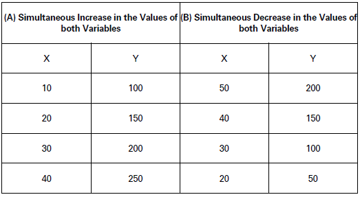
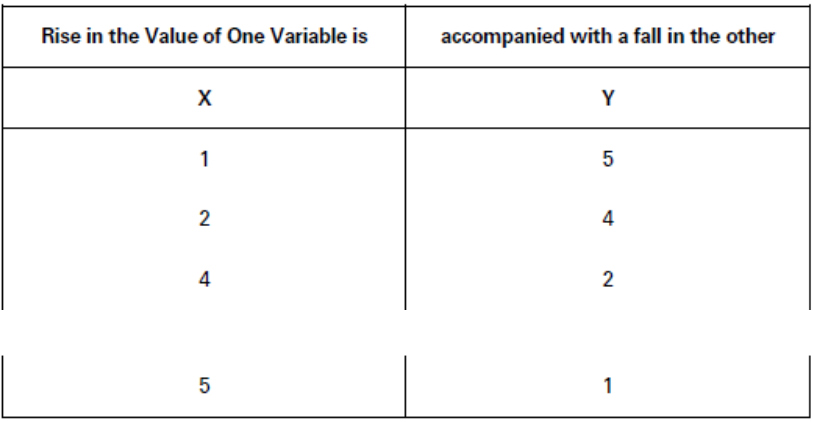
(2) Negative Correlation
When two variables change in different directions, it is called negative correlation. Relationship between price and demand, may be cited as an example. The following table demonstrates this relation:

What does Correlation Measure?
Often the students tend to believe that correlation suggests a relationship between two variables where one is the cause of the other. Example: This is correlation between price and quantity demanded of a commodity. Clearly, an increase in price causes a decrease in quantity demanded, and vice versa. Change in price causes changes in quantity demanded. But to be emphatically noted is the point that cause and effect relationship between the variables is not at all any pre-condition in the theory of correlation.

Correlation just measures the degree and intensity of relationship between the two variables, with or without any cause and effect relationship. Of course, the established relationship between the variables should be capable of offering us some meaningful conclusion. Example: Students who are good in academics may be good in sports also. Certainly, it is a meaningful relationship (or correlation) if one finds it. But surely there is no cause and effect relationship between the two variables. Linear and Non-Linear Correlation
Correlation may be linear or non-linear.

(1) Linear Correlation
When two variables change in a constant proportion, it is called linear correlation. If the two sets of data bearing fixed proportion to each other are shown on a graph paper, their relationship will be indicated by a straight line. Thus, linear correlation implies a straightline relationship.

(2) Non-linear Correlation
When the two variables do not change in any constant proportion, the relationship is said to be non-linear. Such a relationship does not form a straight-line relationship.

Illustration.
Linear Correlatio

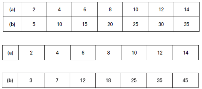
Thus, for every change in variable (a) by 2 units there is a change in variable (b) by 5 units.
Non-linear Correlation

Here there is no specific relationship between the two variables, though both tend to change in the same direction. That is, both are increasing, but not in any constant proportion.

Simple and Multiple Correlation

(1) Simple Correlation
Simple correlation implies the study of relationship between two variables only. Like the relationship between price and demand or the relationship between money supply and price level.

(2) Multiple Correlation
When the relationship among three or more than three variables is studied simultaneously, it is called multiple correlations. In case of such correlation, the entire set of independent and dependent variables is simultaneously studied. For instance, effects of rainfall, manure, water, etc., on per hectare productivity of wheat are simultaneously studied.

The basic difference between Linear and Non-linear Correlation
In case of linear correlation, the two sets of data show some fixed proportion to each other and therefore, form a straight line on a graph paper, in case of nonlinear correlation, the two sets of data do not show any fixed proportion to each other, and therefore, do not make a straight line on a graph paper.

Partial Correlation When more than two variables are involved and out of these the relationship between only two variables is studied treating other variables as constant, then the correlation is partial.

Correlation and Causation
Correlation is a numerical measure of direction and magnitude of the mutual relationship between the values of two or more variables. But the presence of correlation should not be taken as the belief that the two correlated variables necessarily have causal relationship as well. Correlation does not airways arise from causal relationship but with the presence of causa relationship, correlation is certain to exist.

2. DEGREE OF CORRELATION
Degree of correlation refers to the Coefficient of Correlation. There can be the following degrees of positive and negative correlation.
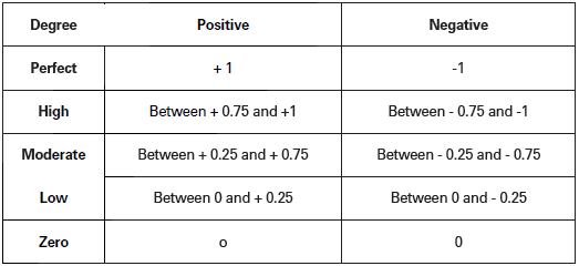
(1) Perfect Correlation: When two variables change in the same proportion it is called perfect correlation. It may be of two kinds:.

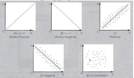
(i) Perfect Positive: Correlation is perfectly positive when proportional change in two variables is in the same direction. In this case, coefficient of correlation is positive (+1).

(ii) Perfect Negative: Correlation is perfectly negative when proportional change in two variables is in the opposite direction. In this case, coefficient of correlation is negative (-1).

(2) Absence of Correlation: If there is no relation between two series or variables, that is, change in one has no effect on the change in other, then those series or variables lack any correlation between them.

(3) Limited Degree of Correlation: Between perfect correlation and absence of correlation there is a situation of limited degree of correlation. In real life, one mostly finds limited degree of correlation. Its coefficient (r) is more than zero and less than one (r > 0 but < 1). The degree of correlation between 0 and 1 may be rated as:

(i) High: When correlation of two series is close to one, it is called high degree of
correlation. Its coefficient lies between 0.75 and 1,

(ii) Moderate: When correlation of two series is neither large nor small, it is called moderate degree of correlation. Its coefficient lies between 0.25 and 0.75.

(iii) Low: When the degree of correlation of two series is very small, it is called low degree of correlation. Its coefficient lies between 0 and 0.25. All these degrees of correlations may be positive or negative.

Degree of Correlatio

3. METHODS OF ESTIMATING CORRELATION
Various methods are available for estimating correlation between different sets of statistical series. Some of the important ones are as under:
(1) Scattered Diagram Method,

(2) Karl Pearson’s Coefficient of Correlation, and
(3) Spearman’s Rank Correlation Coefficient.

Line of Best Fit
Line of Best Fit is the one that passes through the scattered points such that it represents most of these points. Roughly, half of the scattered points should be on either side of the line.

Scattered Diagram
Scattered diagram offers a graphic expression of the directum and degree of correlation.
To make a Scattered Diagram, data are plotted on a graph paper. A dot is marked for each value. The course of these dots would indicate direction and closeness of the variables. Following pictures show some of the possible directions and the degrees of closeness of the variables.

As should be clear from the scattered diagrams, closeness of the dots towards each other in a particular direction indicates higher degree of correlation. If the dots are scattered (showing neither the closeness nor any direction), it is an indication of low degree of correlation.

A Note
Scattered diagram only shows an approximation of the relationship or closeness of two sets of data. Precise measurement of the relationship is not possible.

Merits and Demerits of Scattered Diagram Merits
(i) Scattered diagram is a very simple method of studying correlation between two variables.

(ii) Just a glance at the diagram is enough to know if the values of the variables have any relation or not.
(iii) Scattered diagram also indicates whether the relation is positive or negative.

Demerits
(i) A scattered diagram does not measure the precise extent of correlation.
(ii) It gives only an approximate idea of the relationship.
(iii) It is not a quantitative measure of the relationship between the variables. It is only a qualitative expression of the quantitative change.

Illustration.
The following table gives height and weight of the students of a class. Make a scattered diagram to show if the relationship is positive or negative and if the relationship is strong or weak.

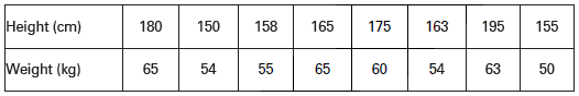
Solution:

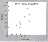
A glance at the above diagram shows that there is positive relationship between height and weight of the students. The dots are moving upward in a particular course from left to right. It shows that with the increase in height, weight also increases.

However, this is a case of limited positive correlation, because the dots do not make any straight line.

Karl Pearson’s Coefficient of Correlation
Scattered diagram method of correlation merely indicates the direction of correlation but not its precise magnitude. Karl Pearson has given a quantitative method of calculating correlation. It is an important and widely used method of studying correlation. Karl Pearsons’ coefficient of correlation is generally written as V.

FORMULA
According to Karl Pearson’s method, the coefficient of correlation is measured as:
𝑟 = Σ𝑥𝑦/𝑁𝜎𝑥𝜎𝑦
where,
r = Coefficient of correlation,
x = X- 𝑋 ̅ .
y =Y- 𝑌 ̅ .
𝜎x = Standard deviation of X series,
𝜎y = Standard deviation of Y series.
N = Number of observations.

This formula is applied only to those series where deviations are worked out from actual average of the series, it does not apply to those series where deviations are calculated on the basis of assumed mean. Value of the coefficient of correlation calculated on the basis of this formula may vary between +1 and -1.
However, the situations, when r = +1, r =-l, or r = 0, are rather rare. Generally, value of V varies between + 1 and – 1.

Note
Karl Pearson’s coefficient of correlation does not apply to those series where deviations are calculated on the basis of assumed mean.
A Modified Version of Karl Pearson’s Formula
In it there is no need to calculate standard deviation of ‘X’ and ‘Y\ Coefficient of correlation may be worked out directly using the following formula:
𝑟 = Σ𝑥𝑦/√Σ𝑥² × Σ𝑦²
Here, x = (X – X̅ ); y = (Y – y̅).

Illustration.
Calculate coefficient of correlation, given the following data:

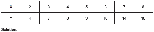
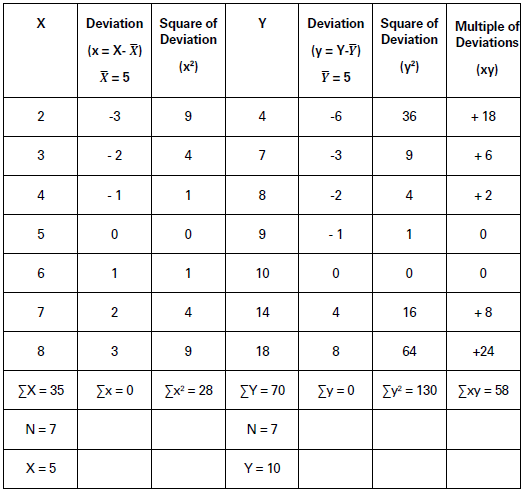
r= Σ𝑥𝑦/√Σ𝑥² × Σ𝑦² ; 𝑥 = (𝑋 − 𝑋̅); 𝑦 = (𝑌 − 𝑌̅)
The table show’s that, Σ𝑥𝑦 = 58,Σ𝑥² = 𝑝8,Σ𝑦² = 130.
Substituting the values, we get
𝑟 = 58/√(28 × 130) = 58/√3,640 =58/60.33 = +0.96
Coefficient of Correlation (r) = + 0.96.
It is a situation of high positive correlation.

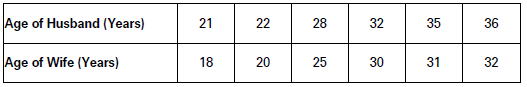
Illustration.
Calculate the coefficient of correlation between the age of husbands and wives.

Solution:

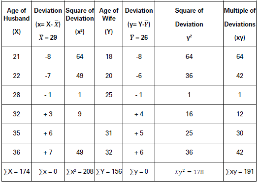
x = (X −X̅ ); y = (Y −Y̅)
X = ΣX/N = 174/6 = 29; Y ¯ = ΣY/N = 156/6 = 26
𝛴𝑥𝑦 = 191, 𝛴𝑥² = 208, 𝛴𝑦² = 178
𝑟 = Σ𝑥𝑦/√Σ𝑥² × Σ𝑦²
r = 191/√208 × 178
=191/√37,024

191/192.42= 0.993
Coefficient of Correlation (r) = 0.993.

Thus, there is a high degree of positive correlation between the age of husband and wife.
Short-cut Method

This method is used when mean value is not in whole number but in fractions. In this method, deviation is calculated by taking the assumed mean of both the series. It involves the following steps:

(i) Any convenient value in X and Y series is taken as assumed mean Ax and Aγ.
(ii) With the help of assumed mean of both the series, deviation of the values of individual variable, i.e., dx (X – Ax) and dy (Y – Aγ) are calculated.
(iii) Σdx and Σdy are found by adding the deviations.
(iv) Deviations of the two series are multiplied, as dx.dy, and the multiples added up to obtain Σdxdy.
(v) Squares of the deviations dx’ and dy2 are added up to find out Σdx2 and Σdy2.
(vi) Finally, coefficient of correlation is calculated using the following formula:

FORMULA
r = Σ𝑑𝑥𝑑𝑦−{(Σ𝑑𝑥)×(Σ𝑑𝑦)/𝑁}/√Σ𝑑𝑥²−(Σ𝑑𝑥)2/𝑁 ×[√Σ𝑑𝑦²−(Σ𝑑𝑦)2/𝑁]

Here,
dx = Deviation of X series from the assumed mean = (X-A),
dy = Deviation of Y series from the assumed mean = (Y – A),
Σdxdy = Sum of the multiple of dx and dy.
Σdx² = Sum of square of dx.
Σdy² = Sum of square of dy.
Σdx = Sum of deviation of X series.
Σdy = Sum of deviation of Y series.
N = Total number of items.

Illustration. 
Calculate coefficient of correlation between the price and quantity supplied.

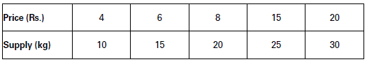
Solution:

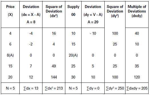
r = {Σ𝑑𝑥𝑑𝑦− (Σ𝑑𝑥)×(Σ𝑑𝑦)/𝑁}/ √(Σ𝑑𝑥2− (Σ𝑑𝑥)2/𝑁) ×√(Σ𝑑𝑦2− (Σ𝑑𝑦)2/𝑁)
=205 − (13) × (0)/5/√(213 − (13)2/5) × √(250 − (0)2/5)
= 205 − 0/√213 − 33.80 × √250 − 0
= 205/√179.20 × √250 = 205/13.39 × 15.81
= 205/211.70
= +0.97

Coefficient of Correlation (r) = + 0.97
This is a situation of a high degree of positive correlation.
Step-deviation Method
The method involves the following steps:

(i) Repeat Step-1 and Step-2 of the short-cut method.

(ii) Now divide ‘dx’ and ‘dy’ by some common factor as dx′ = dx/C1
, dy′ = dy/C2
= here C2 is
common factor for scries X and C2 is common factor for series Y. And dx’ and dy’ are
step-deviations.

(iii) Σdx’ and Σdy’ are found by adding the deviations.

(iv) Deviations of the two series are multiplied, as dx’ × dy’, and the multiples added up
to obtain Σdx’dy’.

(v) Squares of the deviations dx’2 and dy’2 are added up to find out Σdx’2 and Σdy’2.

(vi) Finally, coefficient of correlation is calculated using the following formula:

FORMULA
Σ𝑑𝑥′𝑑𝑦′ − {(Σ𝑑𝑥′) × (Σ𝑑𝑦′)/𝑁}/√{Σ𝑑𝑥′2 − (Σ𝑑𝑥′)2/𝑁} × √{Σ𝑑𝑦′2 − (Σ𝑑𝑦′)2/𝑁}

Illustration.
Calculate coefficient of correlation between the price and quantity demanded.

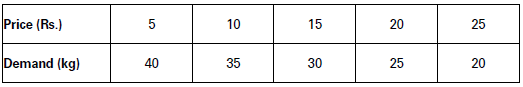
Solution;

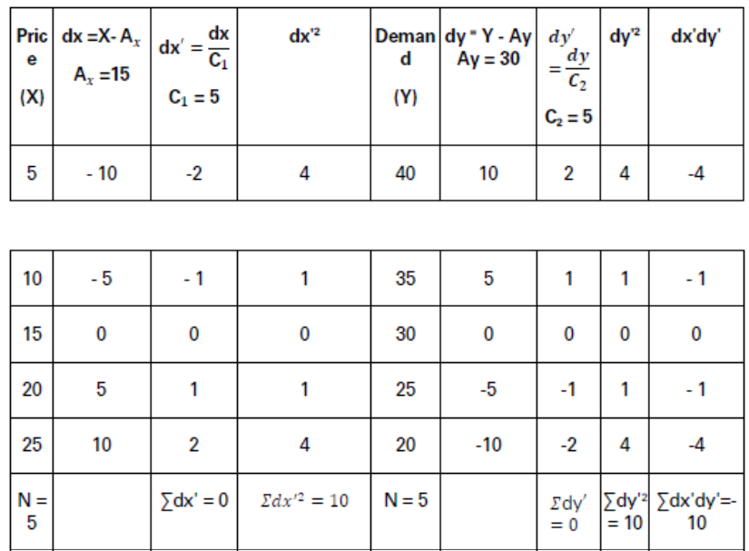
Σ𝑑𝑥′𝑑𝑦′ − (Σ𝑑𝑥′) × (Σ𝑑𝑦′)/𝑁/√{Σ𝑑𝑥′2 − (Σ𝑑𝑥′)2/𝑁} × √(Σ𝑑𝑦′2 − (Σ𝑑𝑦′)2/𝑁)
= −10 −05/√10 −05 × √10 −05
= −10/√10 × √10 = −10/10 = −1
Coefficient of Correlation (r) = – 1.
This is a situation of a perfectly negative correlation between price and quantity demanded.

Properties of Correlation Coefficient
(i) r has no unit. It is a pure number. It means units of measurement are not parts of r.
(ii) A negative value of r indicates an inverse relation, and if r is positive, the two variables move in the same direction.
(iii) If r = 0, the two variables are uncorrelated. There is no linear relation between them. However, other types of relation may be there.
(iv) If r = 1 or r = – 1, the correlation is perfect or proportionate. A high value of r indicates strong linear relationship, i.e., + 1 or -1.
(v) The value of the correlation coefficient lies between minus one and plus one, i.e., -l ≤ r ≤ + l .If the value of r lies outside this range, it indicates error in calculation.

Spearman’s Rank Correlation Coefficient
In 1904, Charles Edward Spearman developed a formula to calculate coefficient of correlation of qualitative variables. It is popularly known as Spearman’s Rank Difference Formula or Method. There are some variables whose quantitative measurement is not

possible. These variables are known as qualitative variables (or more precisely ‘attributes’) such as beauty, bravery, wisdom, ability, virtue, etc.
The attributes cannot be expressed in numbers or quantitative terms. Their relative merit can be determined on the basis of their order of preference or ranking. For instance, in a fancy-dress competition two judges may rank the participants in order of preference. Similarly, the selection committee may prepare a list of successful candidates in order of preference. We experience many such examples in our day-to-day life.

It is in such situations that we use Spearman’s Rank Difference Method.

FORMULA
𝒓𝒌 = 𝟏 − 𝟔Σ𝑫𝟐/𝑵𝟑 − 𝑵

Here.
r = Coefficient of rank correlation.
D = Rank differences.
N = Number of pairs.
We shall study the calculation of rank correlation in three different situations:
(i) When Ranks are given;
(ii) When Ranks are not given; and
(iii) When the values of the series are the same.
Following illustration explains the calculation of Rank Correlation.

Coefficient of Rank Correlation when Ranks are given

Illustration.
Solution:

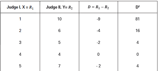
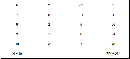
𝑟𝑘 = 1 − 6Σ𝐷2/𝑁3 − 𝑁
Here, N = 10; ΣD2 = 264
𝑟𝑘 = 1 − 6 × 264/(10)3 − 10
= 1 − 1,584/990
= 1 – 1.6 = – 0.6
Coefficient of Rank Correlation (rk) = – 0.6.
There is a negative coefficient of rank correlation to the tune of -0.6 which is fairly high. High negative correlation suggests that two sets of judgements are fairly opposite to each other.

Coefficient of Rank Correlation when Ranks are not given
Sometimes, only data are given and not the ranks. In such situations, ranks are to be accorded by the student himself. While according the ranks, uniform procedure should be adopted for both the series. For example, if the highest rank is accorded to the lowest value in one series, the same must be done for the second series as well.

Illustration.
In a Poetry Recitation Competition, 10 participants were accorded following marks by two different judges, X and Y:

Solution:
There are 10 items each in the two series in this question. We may accord, the highest rank, i.e., 10 to highest value/item in each series, i.e., 18 in series X and 15 in series Y, and accord the lowest rank, i.e., 1 to the lowest value/item in each series, i.e., 9 in series X and 2 in series Y.

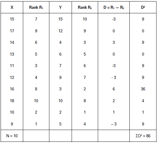
𝑟𝑘 = 1 − 6Σ𝐷2/𝑁3 − 𝑁
Here, 𝑁 = 10; Σ𝐷2 = 86
𝑟𝑘 = 1 − 6 × 86/(10)3 − 10
= 1 − 516/1,000 − 10
= 1 − 0.52
= 0.48

Coefficient of Rank Correlation (rk) = 0.48.
Thus, there is a positive rank correlation of a moderate degree of 0.48.

Coefficient of Rank Correlation when Ranks are Equal
Sometimes, two or more items in the series have equal ranks. In such situations, average of the two ranks (say 7.5 of the ranks 7 and 8) is accorded to each value. But one is likely to commit mistake in this procedure. In order to avoid the possibility of error, the following formula is used for the calculation of coefficient of rank correlation in such situations:

FORMULA
𝑟𝑘 = 1 − 6 [Σ𝐷2 + 1/12 (𝑚1/3 − 𝑚1) + 1/12 (𝑚2/3 − 𝑚2) + ⋯ ] /𝑁3 − 𝑁
Here, m = Number of items of equal ranks.

Illustration.
Calculate coefficient of rank correlation between the marks in Economics and Statistics,
as indicated by 8 answer books of each of the two examiners.

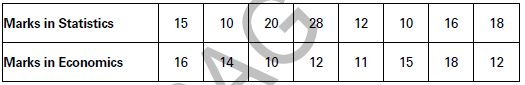
Solution:
There are 8 answer books each in Economics and Statistics indicating different marks.
Rank 1 is accorded to the highest score. In Statistics, two answer books indicate 10 marks each. Hence, the first answer book has been given Rank 8 and the second 7. Thus, the average rank = 8+7/2 = 7.5 has been accorded to both. Likewise, in Economics two answer books indicate 12 marks each. The average rank = 6+5/2 = 5.5 has, therefore, been accorded to both.

Calculation of Coefficient of Rank Correlation

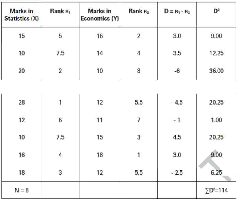
Here, number 10 is repeated twice in series X and number 12 is repeated twice in series Y. Therefore, in X, m = 2 and in Y, m = 2.
𝑟𝑘 = 1 − 6[Σ𝐷2 + 1/12 (𝑚1/3 − 𝑚1) + 1/12 (𝑚2/3 − 𝑚2)] / 𝑁3 − 𝑁
= 1 − 6 [114 + 1/12 (23 − 2) + 1/12 (23 − 2)]/83 − 8
= 1 − 6|114 + 1/12 (6) + 1/12 (6)/512 − 8
= 1 −6 [114 +12+12]/504
= 1 − 6[115]/504
= 1 − 690/504
= 1 − 1.36 = −0.36
Coefficient of Rank Correlation (rk) = – 0.36.

Merits and Demerits of Rank Correlation

Merits
(i) Spearman’s rank correlation method is easier than Pearson’s method of correlation.
(ii) Rank correlation method is very convenient method when the series give only order
of preference and not the actual values of the variables.

(iii) Rank correlation is a superior method of analysis in case of qualitative distributions such as those relating to virtue, wisdom or ignorance.

Demerits

(i) Rank correlation method cannot be used in case of group frequency distributions.

(ii) It can handle only a limited number of observations. It is generally not used when the number of observations exceeds 20.

4. IMPORTANCE OR SIGNIFICANCE OF CORRELATION
Following observations highlight the importance or significance of correlation as a statistical method:

(1) Formation of Laws and Concepts: The study of correlation shows the direction and degree of relationship between the variables. This has helped the formation of various laws and concepts in economic theory, such as, the law of demand and the concept of elasticity of demand.

(2) Cause and Effect Relationship: Correlation coefficient sometimes suggests cause and effect relationship between different variables. This helps in understanding why certain variables behave the way they behave.

(3) Business Decisions: Correlation analysis facilitates business decisions because the trend path of one variable may suggest the expected changes in the other. Accordingly, the businessman may plan his business decisions for the future.

(4) Policy Formulation: Correlation analysis also helps policy formulation. If the Government finds a negative correlation between tax rate and tax collection, it should pursue the policy of low tax rate. Because, low tax rate would lead to high tax collection.