CBSE Class 9 Mathematics Statistics Notes Set 02

BASIC TERMS
Primary data : Data which collected for the first time by the statistical investigator or with the help of his workers is called primary data.

Secondary data : These are the data already collected by a person or a society and these may be in published or unpublished form. These data should be carefully used.

PRESENTATION OF DATA

Raw data : When the data is compiled in the same form and order in which it is collected, it is known as Raw data.

The difference of the highest and the lowest values in the data is called the range of the data.

Frequency : It is a number, which tells that how many times does a particular data appear in a given set of data.

Frequency Distribution :

A tabular arrangement of data showing their corresponding frequencies is called a frequency distribution. The table showing data with their corresponding frequencies is called a frequency table.

Grouped Frequency Distribution :

Consider an example : 100 plants each were planted in 100 schools during Van Mahotsava.
After one month, the number of plants that survived were recorded as :

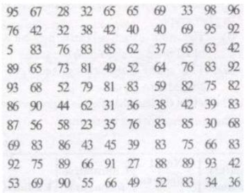
To present such a large *amount of data so that a reader can make sense of it easily, we condense it into groups like 20-29, 30-39, . . 90-99

The data above can be condensed in tabular form as follows:

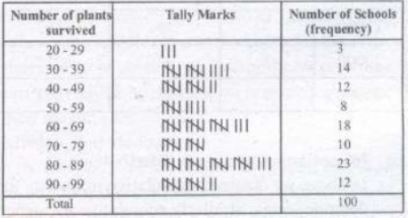
This is called a grouped frequency distribution table.
In each of these classes, the least number is called the lower class limit and the greatest number is called the upper class limit, e.g., in 20-29, 20 is the `lower class limit’ and 29 is the `upper class limit’.

Classes (Class -intervals) : We have groups like 20 – 29, 30 – 39, 90 – 99 in above given example.

Class Mark : The mid-point of a class is called the class mark of the class.

Thus,

Class mark = Upper class limit + Lower class limit / 2

Descrete frequency distribution :

When number of terms is large and variate are descrete, variate can accept some particular values only under finite limits and is repeated then it is called descrete frequency
distribution.

(iii) Continuous frequency distribution :

When number of terms is large and variate is continuous, i.e., variate can accept all values under finite limits and they are repeated then it is called continuous frequency distribution.

CUMULATIVE FREQUENCY

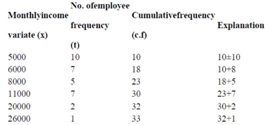
(a) In descrete frequency distribution :

We add all previous frequencies and get cumulative frequency. It will be more clear from the following table :

(b) In continuous frequency distribution :

In above we obtained cumulative frequency for descrete series. Similarly cumulative frequency table can be made from continuous frequency distribution also. For example, for table

Class Frequency Cumulativefrequency (c.f)
0-5 82 82
5-10 92 82+92=174
10-15 53 174+53=227
15-20 27 227+27=254

Here we see that number of students whose age is less than 5 is 82, number of students whose age is less than 10 is 174, number of students whose age is less than 15 is 227 and number of students whose age is less than 20 is 254. Above table can also be written as follows

Class Cumulative frequency (c.f)
Less than 5 82
Less than 10 174
Less than 15 227
Less than 20 254

From this table the number of students of age less than the upper limit of a class, i.e. number of student whose age is less than 5, 10, 15, 20 years – can determined by merely seeing the table but if we need the number students whose age is more than zero, more than 5, more than 10 or more than 15, then table should be constructed as follows :

Frequency Distribution, Cumulatiw FrequencyDistrib ution Cumulativefrequency

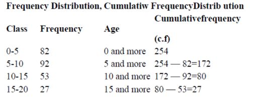
Note : The cumulative frequency of the last class is the total number of frequencies or the total number of observations in the data in the raw form.

GRAPHICAL REPRESENTATION OF DATA

The representation of data through diagrams helps us to visualize the Whole meaning of a numerical distribution at a single glance. There are various methods of representing the data by means of graphs.

(A) Bar graphs
(B) Histograms of uniform width, and of varying widths
(C) Frequency polygons

(1) Bar graph : It is the simplest and most widely used graph in which the numerical data is represented by bars (rectangles) of equal width. . In a bar graph :

(i) The width of each bar can be any, but widths of all the bars should be the same.

(ii) The space between consecutive bars should also be same.
The height (or length) of a bar is proportional to the numerical data it represents.

(2) Histogram : A histogram is a graphical representation of a frequency distribution in the form of rectangles one after the other.

The bases of these rectangles represent the magnitudes of the variables of the class boundaries.
So these are taken along the x-axis.

The heights of these represent the frequencies of the corresponding magnitudes of the variable of the class-boundaries.

(3) Frequency polygon : After drawing the histogram of a frequency distribution, when the mid-points of the respective tops of the rectangles are joined by the line segment, the figure so obtained is known as frequency polygon.

The mid-point of the top of the first rectangle is joined to the mid-point of the earlier interval (imagined) on the x-axis. Similarly the mid-point of the top of the last rectangle is joined to the mid-point of the next interval (imagined) on the x-axis.

Note : If both histogram and frequency polygon are to be drawn, then it is advisable first to draw histogram and then join the mid-points of the tops of the rectangles of the histogram to get frequency polygon.

But if only frequency polygon is to be drawn then first represent the class marks along x-axis and frequencies along y-axis and then plot the point corresponding to the frequency at each class mark.

Note : Frequency polygons can also be drawn independently without drawing histograms. For this, we require the mid-points of the class-intervals used in the data.

These mid-points of the class-intervals are called class-marks.

MEASURES OF CENTRAL TENDENCY (AVERAGES)

There are three main averages :
(1) Mean
(2) Median
(3) Mode

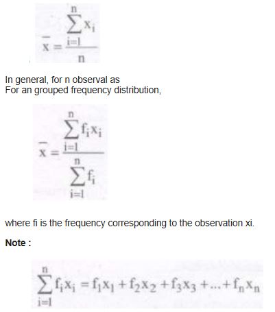
Mean: The mean (or average) of a number of observations is the sum of the values of all the observations divided by the total number of observations.

It is denoted by the symbol x as a’x bar’.

MEDIAN:
The median is that value of the given number of observations, which divides it into exactly two parts.

Median is the middle most or the central value of the variate in a set of observations,when the observations are arranged either in ascending or in descending order of their magnitudes.

Methods to find Median:
When the data is arranged in ascending (or descending) order the median of ungrouped data is calculated as follows:

When the number of observation (n) is odd, the median is the value of the ((n + 1)/2)th observation.

(ii) When the number of observations (n) is even, the median is the mean of the (n/2)th and the n/2 + 1th observations.

MODE:
The mode is that value ofthe observation which occurs most frequently, i.e., an observation with the maximum frequency is called the mode.

Note: It is not effected by presence of extremely large or small items.